Modelling of thermal damage process in soft tissue subjected to laser irradiation



MODELLING OF THERMAL DAMAGE PROCESS IN SOFT TISSUE SUBJECTED TO LASER IRRADIATION

Marek Jasiński

Institute of Computational Mechanics and Engineering
Silesian University of Technology
Gliwice, Poland
marek.jasinski@polsl.pl

Received: 12 April 2018; Accepted: 18 June 2018

Abstract. The numerical analysis of thermal damage process proceeding in biological tissue during laser irradiation is presented. Heat transfer in the tissue is assumed to be transient and two-dimensional. The internal heat source resulting from the laser irradiation based on the solution of the diffusion equation is taken into account. The tissue is regarded as a homogeneous domain with perfusion coefficient and effective scattering coefficient treated as dependent on tissue injury. At the stage of numerical realization, the boundary element method and the finite difference method have been used. In the final part of the paper the results of computations are shown.

MSC 2010: 65M06, 65M38, 80A20

Keywords: bioheat transfer, optical diffusion equation, Arrhenius scheme, boundary element method, finite difference method

1. Introduction

It is known that biological tissues are characterized by a strong scattering and weak absorption in the so-called therapeutic window (wavelengths 650¸1300 nm) [1-4]. Because of this, to describe the light propagation in biological tissues the different mathematical models can be taken into account. One of them is the transport theory which concerns the transport of light through scattering and absorbing media. In this case the radiative transport equation should be considered [4-6]. To solve this equation, different approaches are used: the modifications of discrete ordinates method, the statistical Monte Carlo method or the optical diffusion equation [2, 5, 7].

Interactions between tissue and the laser beam often lead to the temperature elevation that can cause irreversible damage of the tissue. This in turn could cause the alteration of thermophysical and optical properties of tissue, e.g the perfusion coefficient is often treated as the main indicator of tissue injury. In addition, an increase of scattering due to tissue denaturation has a visual effect of tissue “whitening”. Consequently, parameters applied in mathematical models of heat transfer in biological tissue domain can be regarded as tissue damage-dependent [8-11].

The most popular model of the tissue damage process is the Arrhenius injury integral [12-16]. This approach basically refers only to the irreversible tissue damage, however, there are models that allow one to take into account the withdrawal of tissue injury in the case of temporary, small local increasing of temperature [17].

The purpose of this paper is to analyze the phenomena occurring in the laser-treated biological tissue. The analysis is based on the Pennes bioheat transfer equation which is still the most frequent used model to determine the temperature distribution in biological tissues [9, 10, 13, 18], while the light distribution in biological tissue is estimated on the base of the optical diffusion equation [4, 5, 16]. The degree of tissue damage is calculated by using of Arrhenius scheme with TTIW algorithm and two parameters of the tissue are assumed to be dependent on the injury integral (perfusion coefficient and the effective scattering coefficient).

2. Governing equations

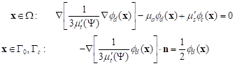
The transient heat transfer in the 2D homogeneous biological tissue domain of rectangular shape W (Fig. 1) is described by the Pennes bioheat transfer equation with adequate boundary-initial conditions [11, 18]

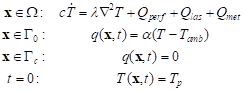where λ [Wm^-1K^-1] is the thermal conductivity, c [Jm^-3K^-1] is the volumetric specific heat, T = T(x, t) is the temperature while denotes its time derivative. The components Q_perf, Q_las and Q_met [Wm^-3] are the internal source functions containing information connected with the perfusion, metabolism and laser irradiation. In boundary-initial conditions, a [Wm^-2K^-1] is the convective heat transfer coefficient, T_amb is the temperature of surroundings while T_p denotes the initial distribution of temperature.

The metabolic heat source Q_met [Wm^–3] is assumed as a constant value while the perfusion heat source is described by the formula

where c_B [Jm^–3K^–1] is the volumetric specific heat of blood, T_B corresponds to the arterial temperature while w(Y) [s^–1] is the perfusion coefficient defined as [8, 9, 17]

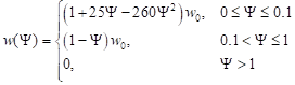where w₀ is the initial perfusion coefficient while Y denotes the Arrhenius injury integral, in form [9, 10, 12]

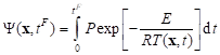where R [J mole^–1K^–1] is the universal gas constant, E [J mole^–1] is the activation energy, P [s^-1] is the pre-exponential factor. A value of integral Y(x) = 1 corresponds to a 63% probability of cell death at a specific point x, while Y(x) = 4.6 corresponds to a 99% probability of cell death at this point. Both values are used as the necrosis criteria.

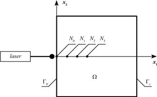
Fig. 1. The domain considered

According to the values of formula , the values of coefficients for the interval from 0 to 0.1 in equation respond to the initial increase of the perfusion coefficient caused by vasodilatation, while values of coefficients for the interval 0.1 to 1 correspond to the decrease of the perfusion during the damage process of the vascular network [9].

The main assumption of the Arrhenius formula is that the damage of tissue is irreversible, so even in the case of very little rise and lowering of temperature the tissue remain damaged. On the other hand, at the initial tissue heating, when the temperature is moderate (i.e. between 37°C and 45¸55°C), the blood vessels in the tissue become dilated without being thermally damaged. Because of this, the TTIW algorithm (thermal tissue injury withdrawal algorithm) has been applied which allows to take into account the possibility of withdrawal of tissue injury when the thermal impulse is ceased [17].

The TTIW algorithm requires the assumption of a certain value Ψ_rec which is defined as recovery threshold. The withdrawal of tissue damage is possible only for those points of the domain considered in which the value of injury coefficient Ψ is below Ψ_rec. If the tissue damage at the point x Î W achieves the value greater than Ψ_rec then the injury becomes irreversible, so, it will be calculated on the base of the Arrhenius formula . The full description of the TTIW algorithm could be found in [17].

The thermal damage of the tissue also affects the optical properties of the tissue. During the process of coagulation, the changes in tissues lead to higher scattering while the absorption remains the same, thus in the current work, the effective scattering coefficient of tissue is described as [10]

where m¢_{s nat} and m¢_{s den} [cm^-1] denote the effective scattering coefficient for native and destructed (denaturated) tissue, respectively.

The source function Q_las (c.f. equation ) associated with the laser heating is defined as follows [2]

where m_a [m^–1] is the absorption coefficient, f_c and f_d are the collimated and diffuse parts of the total light fluence rate, respectively while p(t) is the function equal to 1 when the laser is on and equal to 0 when the laser is off.

The collimated fluence rate part f_c is determined on the basis of the Beer- -Lambert law, namely [2, 11, 16]

where f₀ [Wm^–2] is the surface irradiance of laser, d is the diameter of laser beam and m¢_t [m^–1] is the attenuation coefficient given as

To determine the diffuse fluence rate f_d the optical diffusion equation should be solved [1-3]

where n is the outward unit normal vector.

3. Method of solution

At the stage of numerical realization, the 1^st scheme of the boundary element method (BEM) for 2D transient heat diffusion has been used while the optical diffusion equation has been solved by the finite difference method (FDM).

For the transient heat diffusion problem, for the time grid with constant step Dt, the boundary integral equation corresponding to transition t ^f–1 ® t ^f is of the form

where Q_V denotes the sum of the internal heat function associated with the perfusion, metabolism and laser irradiation (c.f. equation ), T^* is the fundamental solution

where r is the distance from the point under consideration x to the observation point x, a = l/c, while

and B(x) is the coefficient from the interval (0, 1).

In this paper, the constant boundary element has been used. Details concerning numerical realization of the BEM can be found, among others, in [11, 19-21].

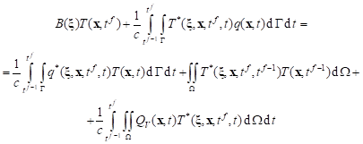
In order to determine the source function Q_las at the internal nodes (c.f. equation ), at each time step additionally the optical diffusion equation must be solved. As it was mentioned previously, it is done by using the finite difference method. The global and local numeration of the nodes is shown in Figure 2.

The difference equation for the central node of stencil can be written in the form

where R_0e are resistances between the central node and remaining nodes of the stencil - Figure 2.

More details concerning numerical realization of the FDM, can be found in [16, 22, 23].

Fig. 2. Five-point stencil and discretization

4. Results of computations

The aim of the research was to analyse the destructive changes in the tissue domain of the size of 4´4 cm during laser irradiation (c.f. Fig. 1). The interior of the domain has been divided into 1600 internal constant cells while the external boundary into 160 constant elements.

The most commonly used types of laser impulses in medical treatments are multiple impulses of duration ranging from a few to several dozen seconds with appropriate pauses between subsequent impulses. The purpose of this is not to overheat, and thus not to cause thermal damage to healthy tissue adjacent to the treated area. Thermography techniques are also used for similar reasons. They allow one to maintain the tissue surface temperature in a certain range and to control the laser action during the medical procedure [1, 5, 10, 13]. Because of this, in current paper, the two cases of laser irradiation were taken under consideration. In example 1, the tissue is subjected to multiple laser impulse (100 seconds on and 100 seconds off) while in example 2 the laser action depends on the tissue surface temperature, meaning the laser is on when the temperature drop below T_ctrl – DT_ctrl and off when the temperature reaches above T_ctrl + DT_ctrl.

In computations, the following values of parameters have been assumed: l = 0.609 Wm^-1K^-1, c = 4.18 MJm^-3K^-1, w₀ = 0.00125 s^–1, m_a = 0.4 cm^–1, m¢_{s nat} = 10 cm^–1, m¢_{s den} = 40 cm^–1, Q_met = 245 Wm^–3, c_B = 3.9962 MJm^-3K^-1, T_B = 37°C, P = 3.1×10⁹⁸ s^–1, E = 6.27×10⁵ Jmole^–1, R = 8.314 Jmole^–1K^–1, Y_rec = 0.05, ϕ₀ = 30 Wcm^–2, d = 2 mm, a = 10 Wm^–2K^–1, T_amb = 20°C, T_p = 37°C, T_ctrl ± DT_ctrl = 70±3°C, Dt = 1 s [10, 11, 17].

The optical parameters of tissue (m_a, m¢_{s nat} and m¢_{s den}), which were assumed in simulations, are typical for near-IR irradiation on soft tissue like e.g. Nd:YAG laser of 1064 nm which is used for prostate coagulation.

The results containing information about courses in time are presented in points N₀(0,0), N₁(0.0045,0), N₂(0.0065,0), N₃(0.0085,0).

In Figure 3, distribution of the diffuse fluence rate obtained on the basis of the optical diffusion equation is shown. It is visible that initially the area of scattering is larger, although the values of f_d are lower than they are in the end of the simulation. The results are presented for example 1 only, but it should be pointed out that in example 2 they were almost the same.

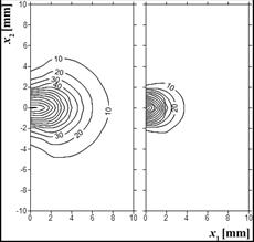
Fig. 3. Distribution of diffuse fluence rate ϕ_d [kWm^–2] for 0 and 500 s (example 1)

Figures 4 and 5 are associated with tissue temperature. In Figure 4, the temperature history for the point N₀ and both examples analyzed are presented. For multiple laser impulse (example 1), it is visible that for each of the subsequent laser’s cycle (on/off), the reached temperatures are higher and higher. Lower temperatures obtained for the example 2 are also visible in Figure 5.

Fig. 4. Tissue temperature history at the node N₀ (examples 1 and 2)

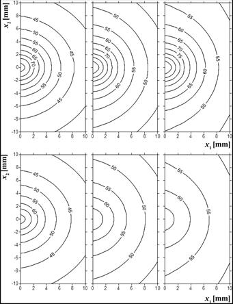
Fig. 5. Temperature distribution [°C], time 100, 300, 500 s (up: example 1, down: example 2)

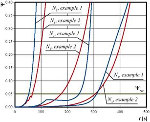
Fig. 6. Arrhenius injury integral history at nodes N₁, N₂, N₃ (examples 1 and 2)

In Figure 6, the time courses of the Arrhenius integral. The decreases of the Arrhenius integral value resulting from the application of the TTIW algorithm were noticed: for example 1 at point N₂ while for example 2 at point N₁. In example 2, they are not big, but they are still visible.

Figure 7 shows the distribution of the Arrhenius injury integral for times 100, 300 and 500 s for both examples. The differences are visible mainly at the early stage of the tissue damage process.

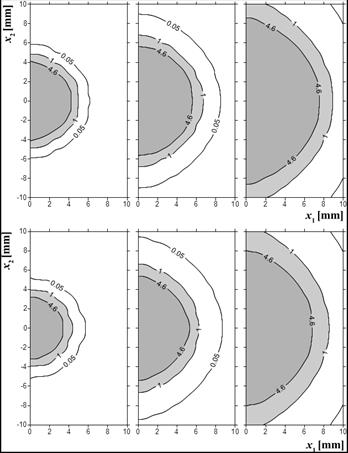
Fig. 7. Arrhenius injury integral distribution, time 100, 300, 500 s (up: example 1, down: example 2)

Obviously, all changes in the value of the Arrhenius integral have reflection in changes of tissue damage-dependent parameters assumed in the current model, i.e. perfusion coefficient and effective scattering coefficient. The distribution of these parameters is presented in the next two figures.

In Figure 8, the grey zone refers to the zone in which the value of the perfusion coefficient is lowered while the check zone is the so-called hyperemic ring - the area in which the value of perfusion is raised. As it can be seen, this zone is almost adjacent to the coagulation zone. In Figure 9, the distribution of the effective scattering coefficient is presented.

In Figure 10, the information about expansion of tissue damage is presented. The number of elements on the scale of the figure means that tissue injury is treated as a sum of element on which the injury integral is above 0.01, so this value could be treated as the border of thermally untouched tissue.

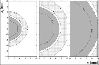
Fig. 8. Perfusion coefficient distribution w(Y) ´ 1000 [s^–1], time 100, 300, 500 s (example 2)

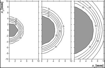
Fig. 9. Effective scattering coefficient m¢_s(Y) [cm^–1], time 100, 300, 500 s (example 2)

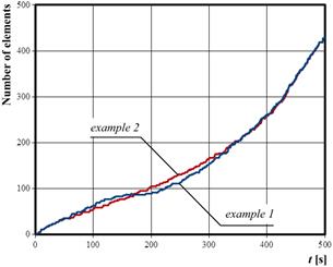
Fig. 10. Expansion of the thermal injury

6. Conclusion

The heat transfer process in the tissue subjected to laser irradiation is analyzed. The analysis is based on the bioheat transfer equation in the Pennes formulation while for calculation of light distribution in tissue, the Beer-Lambert law (collimated part of fluence rate) and optical diffusion equation (diffuse part of fluence rate) are used. The perfusion coefficient and effective scattering coefficient are assumed to be dependent on the tissue damage which was estimated on the base of Arrhenius injury integral with the TTIW algorithm. Because the calculation in this way is closer to real conditions of the tissue destruction process during laser-tissue interaction, the estimation of the total size of tissue damage is more precise.

Comparing the process of increasing of tissue damage, it is visible that for the example 2 the expansion of the lesion occurs slightly more evenly. The final areas of tissue damage are almost the same in both cases (c.f. Figure 10), however in the example 2 it was achieved at a lower local temperature value (c.f. Figures 4 and 5).

It should be pointed out that for the description of light propagation in tissue, different models could also be taken into account e.g. the Monte Carlo approach [7]. It is also possible to use another equation of bioheat transfer such as Cattaneo- -Vernotte equation or dual phase lag equation [4, 5, 14, 15, 20-22, 24]. Furthermore, due to individual characteristics of biological objects, the various values of thermophysical and optical parameters should be considered. For this purpose, for example, the sensitivity analysis can be used.

Acknowledgements

The research is funded from the projects Silesian University of Technology, Faculty of Mechanical Engineering.

References

[1] Welch, A.J., & van Gemert, M.J.C. (Eds.) (2011). Optical-thermal Response of Laser Irradiated Tissue. Springer.

[2] Niemz, M.H. (2007). Laser-tissue Interaction. Berlin, Heidelberg, New York: Springer-Verlag.

[3] Tuchin, V.V. (2007). Tissue Optics: Light Scattering Methods and Instruments for Medical Diagnosis (Vol. PM166). Bellingham: SPIE Press.

[4] Dombrovsky, L.A. (2012). The use of transport approximation and diffusion-based models in radiative transfer calculations. Computational Thermal Sciences, 4(4), 297-315.

[5] Dombrovsky, L.A., Randrianalisoa, J.H., Lipinski, W., & Timchenko, V. (2013). Simplified approaches to radiative transfer simulations in laser induced hyperthermia of superficial tumors. Computational Thermal Sciences, 5(6), 521-530.

[6] Jacques, S.L., & Pogue, B.W. (2008). Tutorial on diffuse light transport. Journal of Biomedical Optics, 13(4), 1-19.

[7] Banerjee, S., & Sharma, S.K. (2010). Use of Monte Carlo simulations for propagation of light in biomedical tissues. Applied Optics, 49, 4152-4159.

[8] Jasiński, M. (2011). Numerical modeling of tissue heating with application of sensitivity methods. Mechanika 2011: Proceedings of the 16th International Conference, 137-142.

[9] Abraham, J.P., & Sparrow, E.M. (2007). A thermal-ablation bioheat model including liquid-to-vapor phase change, pressure- and necrosis-dependent perfusion, and moisture-dependent properties. International Journal of Heat and Mass Transfer, 50(13-14), 2537-2544.

[10] Glenn, T.N., Rastregar, S., & Jacques, S.L. (1996). Finite element analysis of temperature controlled coagulation in laser irradiated tissue. IEEE Transactions on Biomedical Engineering, 43(1), 79-86.

[11] Jasiński, M. (2018). Numerical analysis of soft tissue damage process caused by laser action. AIP Conference Proceedings, 1922, 060002.

[12] Henriques, F.C. (1947). Studies of thermal injuries, V. The predictability and the significance of thermally induced rate process leading to irreversible epidermal injury. Archives of Pathology, 43, 489-502.

[13] Fasano, A., Hömberg, D., & Naumov, D. (2010). On a mathematical model for laser-induced thermotherapy. Applied Mathematical Modelling, 34(12), 3831-3840.

[14] Narasimhan, A., & Sadasivam, S. (2013). Non-Fourier bio heat transfer modelling of thermal damage during retinal laser irradiation. International Journal of Heat and Mass Transfer, 60, 591-597.

[15] Mochnacki, B., & Majchrzak, E. (2017). Numerical model of thermal interactions between cylindrical cryoprobe and biological tissue using the dual-phase lag equation. International Journal of Heat and Mass Transfer, 108(1-10), 2017.

[16] Jasiński, M., Majchrzak, E., & Turchan, L. (2016). Numerical analysis of the interactions between laser and soft tissues using generalized dual-phase lag model. Applied Mathematical Modelling, 40(2), 750-762.

[17] Jasiński, M. (2015). Modelling of thermal damage in laser irradiated tissue. Journal of Applied Mathematics and Computational Mechanics, 14, 67-78.

[18] Paruch, M. (2017), Identification of the cancer ablation parameters during RF hyperthermia using gradient, evolutionary and hybrid algorithms. International Journal of Numerical Methods for Heat & Fluid Flow, 27, 674-697.

[19] Brebia, C.A., & Dominquez, J. (1992). Boundary Elements, an Introductory Course (Computational Mechanics Publications). London: McGraw-Hill Book Company.

[20] Majchrzak, E., & Turchan, L. (2015). The general boundary element method for 3D dual-phase lag model of bioheat transfer. Engineering Analysis with Boundary Elements, 50, 76-82.

[21] Majchrzak, E. (2010). Numerical solution of dual phase lag model of bioheat transfer using the general boundary element method. CMES: Computer Modeling in Engineering & Sciences, 69(1), 43-60.

[22] Majchrzak, E., & Mochnacki, B. (2016). Dual-phase lag equation. Stability conditions of a numerical algorithm based on the explicit scheme of the finite difference method. Journal of Applied Mathematics and Computational Mechanics, 15, 89-96.

[23] Majchrzak, E., Turchan, L., & Dziatkiewicz, J. (2015). Modeling of skin tissue heating using the generalized dual-phase lag equation. Archives of Mechanics, 67(6), 417-437.

[24] Xu, F., Seffen, K.A., & Lu, T.J. (2008). Non-Fourier analysis of skin biothermomechanics. International Journal of Heat and Mass Transfer, 51(9-10), 2237-2259.