Graph presentation of binary strings

• BibTex
• RIS
• APA
• Harvard
• IEEE
• MLA
• Vancouver
• Chicago

@article{Gjonbalaj_2018,
   doi = {10.17512/jamcm.2018.2.02},
   url = {https://doi.org/10.17512/jamcm.2018.2.02},
   year = 2018,
   publisher = {The Publishing Office of Czestochowa University of Technology},
   volume = {17},
   number = {2},
   pages = {17--27},
   author = {Qefsere Doko Gjonbalaj and  Valdete Rexhëbeqaj Hamiti},
   title = {Graph presentation of binary strings},
   journal = {Journal of Applied Mathematics and Computational Mechanics}
}

TY  - JOUR
DO  - 10.17512/jamcm.2018.2.02
UR  - https://doi.org/10.17512/jamcm.2018.2.02
TI  - Graph presentation of binary strings
T2  - Journal of Applied Mathematics and Computational Mechanics
JA  - J Appl Math Comput Mech
AU  - Gjonbalaj, Qefsere Doko
AU  - Hamiti, Valdete Rexhëbeqaj
PY  - 2018
PB  - The Publishing Office of Czestochowa University of Technology
SP  - 17
EP  - 27
IS  - 2
VL  - 17
SN  - 2299-9965
SN  - 2353-0588
ER  - 

Gjonbalaj, Q., & Hamiti, V. (2018). Graph presentation of binary strings. Journal of Applied Mathematics and Computational Mechanics, 17(2), 17-27. doi:10.17512/jamcm.2018.2.02

Gjonbalaj, Q. & Hamiti, V., 2018. Graph presentation of binary strings. Journal of Applied Mathematics and Computational Mechanics, 17(2), pp.17-27. Available at: https://doi.org/10.17512/jamcm.2018.2.02

[1]Q. Gjonbalaj and V. Hamiti, "Graph presentation of binary strings," Journal of Applied Mathematics and Computational Mechanics, vol. 17, no. 2, pp. 17-27, 2018.

Gjonbalaj, Qefsere Doko, and Valdete Rexhëbeqaj Hamiti. "Graph presentation of binary strings." Journal of Applied Mathematics and Computational Mechanics 17.2 (2018): 17-27. CrossRef. Web.

1. Gjonbalaj Q, Hamiti V. Graph presentation of binary strings. Journal of Applied Mathematics and Computational Mechanics. The Publishing Office of Czestochowa University of Technology; 2018;17(2):17-27. Available from: https://doi.org/10.17512/jamcm.2018.2.02

Gjonbalaj, Qefsere Doko, and Valdete Rexhëbeqaj Hamiti. "Graph presentation of binary strings." Journal of Applied Mathematics and Computational Mechanics 17, no. 2 (2018): 17-27. doi:10.17512/jamcm.2018.2.02

GRAPH PRESENTATION OF BINARY STRINGS

Qefsere Doko Gjonbalaj, Valdete Rexhëbeqaj Hamiti

Department of Math, Faculty of Electrical and Computer Engineering
University of Prishtina “Hasan Prishtina”
Prishtinë, 10 000, Kosovë
qefsere.gjonbalaj@uni-pr.edu, valdete.rexhebeqaj@uni-pr.edu

Received: 31 January 2018; Accepted: 26 April 2018

Abstract. This article is motivated by the problem of finding a graph, which operates on the principle of the Hasse diagram. In the present article, the Hasse diagram technique (HDT) was applied to relate binary string sets with graph theory. We investigate this relation in detail and propose a new graph, the so-called 2n-Parallel Graph , and an efficient pseudo code that decompresses a given binary string set to its elements. The goal of this pseudo code is its application in determining the number of strings with a certain number of first bits consecutive 1’s (0’s). This pseudocode is also responsible for the solution of several combinatorial problems on a certain binary string. Furthermore, our results are valid for any string length.

MSC 2010: 05C90, 68R10

Keywords: Hasse diagram, binary strings

1. Introduction

As we know, binary strings can be decoded using a binary tree. To read that string from any prescribed position forward, one starts at the root and moves down from the root of the tree to the external node that holds that character: a 0 bit identifies a left branch in the path, and a 1 bit identifies a right branch. This procedure is continued until the bit string of length n is decoded. But with an increase in the length of the string, the binary tree becomes more complicated [1].

So we look for another way to represent binary strings that will allow us to minimize the number of branches in our drawing. Looking to simplify the problem we have defined a new graph that works by use of the Hasse diagram technique.

2. Basic notions

All graphs considered here are simple, finite, connected and undirected. We follow the basic notions and terminologies of graph theory as in [1].

Definition 2.1. A graph consists of two sets; called vertex set of and called edge set of . More precisely we denote the vertex set of as ) and the edge set of as . Elements of and are called vertices and edges, respectively. The number of vertices in is denoted by and the number of edges in is denoted by .

Definition 2.2. A walk in which no vertex is repeated is called a simple path. A path with vertices is denoted as .

Definition 2.3. A graph is connected if there is a path between every pair of vertices of . A graph, which is not connected, is called a disconnected graph.

Definition 2.4. [2] A graph with vertices is called a path if has exactly two vertices with degree 1 and exactly vertices with degree 2.

Definition 2.5. A simple path in a graph that passes through every vertex exactly once is called a Hamilton path, and a simple circuit in a graph that passes through every vertex exactly once is called a Hamilton circuit.

Theorem 2.1. [3] Let be a finite connected graph on n vertices. Then contains at least edges, with equality if and only if is a tree.

Here we review some basic definitions and notions concerning posets (partially ordered set) and the Hasse diagram.

Definition 2.6. [2] A Hasse diagram is a directed graph representation of a poset whose vertices represent elements of and whose directed edges signify the relation. That is, an edge means

In other words, the Hasse diagram of poset is defined:

(1)

(2)

and in this case we say that covers , so that the line segment from to runs upwards .

If we assume that all edges are pointed “upward”, we do not have to show the directions of the edges.

The objects (vertices) in a Hasse diagram that are not covered by other objects are called “maximal objects.” Objects that do not cover other objects are called “minimal objects.” In some diagrams there are also isolated objects that can be considered as maximal and minimal objects at the same time. A chain (string) is a set of comparable objects; therefore levels can be defined as the longest chain within the diagram. An antichain is a set of mutually incomparable objects, located at one and the same level. The height of the diagram is the longest chain, and the longest antichain is its width [4].

3. 2n Parallel Graph (2nPG)

Let be the set Then the set of all finite binary strings of length is written as can be ordered by the prefix relation: for is a prefix of if either or is a finite initial substring of . We write if is a prefix of and if neither nor is a prefix of the other (some authors write ). For each set of binary strings of length there is

For brevity, we give the following definition.

Definition 3.1. [5] Let be an element of Weight of , denoted by is defined as

For example, the string 10011 has weight 3.

Now we are going to define an efficient graph (which operates on the principle of Hasse diagram) for the set of binary strings of length whose weight (number of 1s) are in the range where

Definition 3.2. Parallel Graph is a graph consisting of vertexes situated in the proportional way in to parallel line. The vertices in first line will be denoted with where and for while vertices in second line with where and for The set of edges in graph will be defined with for and all edges are pointed “upward”, which means it works by the Hasse diagram technique.

From the definition of graph it follows that the set of vertices are defined by and

The problem of enumeration of all n-bit binary strings is equivalent to finding a Hamilton path in the graph. Because of the Hasse diagram technique, the Hamilton path in graph contains only n vertices (not 2n).

Thinking of binary strings as path in the graph, based on Theorem 1.1, the strings of length are mapped to a path of length . So, from this fact we conclude that:

Theorem 3.1. Let be the set of all finite binary strings of length , where Then, the graph , which represents the element of set for has edges, which means that

Proof: From the definition 3.2, the set of edges of graph is the set for Therefore, from the Theorem 1.1, every subset of set will have edges and since has four such subsets then follows that

Following, based on the definition 3.2, we will construct a graph and compare it with binary trees. By representing the set of binary strings with both graphs: with and by binary tree, we can see the advantages and simplicity of the first graph to the second graph.

Example 3.1. We are going to present the set of binary strings with the graphs and with the binary trees, for Here, for the graph we will use the Hasse diagram technique.

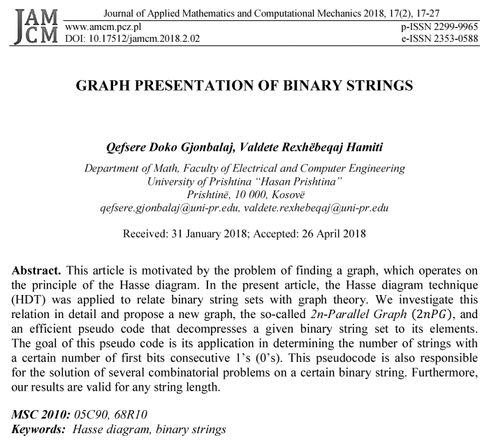
For we have (Fig. 1a and 1b):

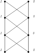
Fig. 1a. graph for binary strings of length

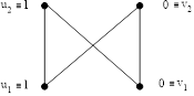
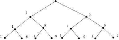
Fig. 1b. Binary tree for binary strings of length

In this case we get binary strings: 11, 10, 01, 00.

For we have (Fig. 2a and 2b):

Fig. 2a. graph for binary strings of length

Fig. 2b. Binary tree for binary strings of length

In this case we get binary strings:

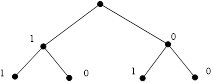
For we have (Fig. 3a and 3b):

Fig. 3a. graph for binary strings of length

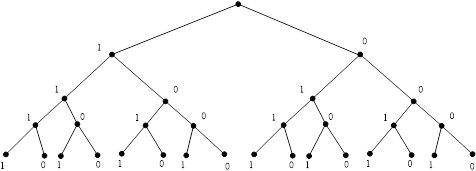
Fig. 3b. Binary tree for binary strings of length

In this case we get binary strings: 1111, 1110, 1101, 1100, 1011, 1001, 1010, 1000, 0000, 0001, 0010, 0011, 0100, 0110, 0101, 0111.

We can continue to construct, for each , a Hamilton path in a graph with the following additional property: edges between levels and of a graph must appear on the path before edges between levels and

Corollary 3.1. Let be the set of all finite binary strings of length , where Then, for the number of edges of a graph creates the arithmetic sequence while the number of edges in a binary tree creates the sequence .

Proof: From the example 3.1, we note that the sequence of number of a graph is: or the arithmetic sequence with first element and difference (it can be proved with mathematical induction). Also the number of edges of binary trees creates the sequence:

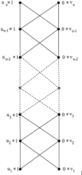
Fig. 4. graph for binary strings of length

Corollary 3.2. Let be the set of all finite binary strings of length , where Then, the number of vertices of a graph creates the arithmetic sequence while the number of vertices of binary trees creates the sequence

Proof: From the example 3.1, we note that the sequence of number of vertices of a graph is: or the arithmetic sequence with first element and difference (it can be proved with mathematical induction). Also the number of edges of binary trees creates the sequence:

In conclusion, based on two corollaries and our own example we can see that the graph, is much more practical because it has a much smaller number of vertices and edges compared with the binary tree, in which the number of vertices and edges is much larger, and it grows very fast. Also, the advantage of this graph is the fact that it is easier to draw and takes less space.

In following we will describe the pseudo code that produces a graph.

4. Pseudocode of a 2n Parallel Graph

In this section an efficient pseudocode will be provided that produces a graph by decompressing a given binary string set to its elements and how does it operates on the principle of Hasse diagram. At the beginning, we give a pseudo-code and afterwards, we discuss the complexity of our solution.

The problem of enumeration of all n-bit binary strings is equivalent to finding a Hamilton path with n vertices and edges, in the graph, which means that at the same time we will determine the binary strings and Hamiltonian paths.

In that case, we denote with all binary strings of length where the first bits are consecutive 1’s (0’s).

Our pseudocode for the Parallel Graph is presented as a method called 2NPG(n) (cf. Fig. 5) which takes as a parameter the length for each of the binary strings that are to be generated.

2NPG(n)

INPUT: n is the length of each of the binary strings to generate.

OUTPUT: S is the set of generated binary strings S_kⁿ such that

· each S_kⁿ is represented with [e₁,e₂,e₃,..,e_k–1,e_k,e_k+1,..,e_n–1,e_n], and

1 let initially S ß {} // initially is S an empty set of binary strings

2 for k ß n to 1 // for each step below, i.e. distinct nr. of consecutive 1’s

3 do 2nPG(n, k) // where k <= n

4 RETURN {S_kⁿ}ß {[e₁,e₂,e₃,…,e_k–1,e_k,{e_k+1,...,e_n–1,e_n}]}

5 RETURN S ß S U{S_kⁿ}ß {[e₁,e₂,e₃,…,e_k–1,e_k,e_k+1,...,e_n–1,e_n]}

Fig. 5. The 2NPG(n) pseudocode

We represent with [e₁,e₂,e₃,.., e_k-1,e_k,e_k+1,..,e_n-1,e_n] each of the binary strings S_kⁿ of length n to be generated as elements of the final set S of all binary strings generated at the output. The S set which is initially an empty set (line 1 in the pseudo-code) is progressively extended (line 5) for each possible k as first consecutive 1 bits (line 2) in the strings to generate by recursively invoking the 2NPG(n, k) method (line 3 to 4).

2NPG(n, k)

INPUT:

· n is the length of each of the binary strings to generate

· k represents the nr. of first bits consecutive 1’s in the strings to generate.

OUTPUT: S is the set of generated binary strings S_kⁿ such that

· each S_kⁿ is represented with [e₁,e₂,e₃,…,e_k–1,e_k,e_k+1,...,e_n–1,e_n].

1 let initially {S_kⁿ} ß {} // initially is {S_kⁿ} an empty set of binary strings

2 for i ß 1 to k

3 do e_iß u_i // assign 1 to e_i since u’s are always 1’s

4 if k ≠ n then e_k+1ß v_k+1 // assign 0 to e_i+1 since v’s are always 0’s

5 if k < n–1 then for i ß k+1 to n

6 do 2nPG(n’) // where n’ = n–k; each S is S_k’^n’ß[e_k+1,..,e_n–1,e_n]

7 RETURN {S_k’^n’}ß {[e_k+1,...,e_n–1,e_n]}

8 RETURN {S_kⁿ}ß {S_kⁿ} U {[e₁,e₂,e₃,…,e_k–1,e_k,{e_k+1,...,e_n–1,e_n}]}

Fig. 6. The 2NPG(n, k) pseudocode

It is obvious that in the very first iteration of the outer for loop in the 2NPG(n) pseudocode above where makes the inner for loop in 2NPG(n, k) (lines 3 to 4) generate a string of length n with all 1’s, i.e. the string S_nⁿ :

since lines 5 and 6 to 8 fail due to conditions in line 5 and line 6 evaluating to false.

Next, due to (refer again to outer for loop in 2NPG(n), this time its second iteration), the inner for loop in 2NPG(n, k) (lines 3 to 4) will generate a string with 1’s, whereas the last bit of the string will be set to 0 (line 5) since the condition in line 5 evaluates to true, i.e. the following string S_n–1ⁿ: will be generated at the output:

Note that lines 6 to 8 fail due to condition in line 6 evaluating to false.

In every other next iteration of the outer for loop in 2NPG(n) starting from the 3^rd iteration, i.e., for to both conditions (lines 5 and 6) in the inner for loop in 2NPG(n, k) are evaluated to true. As a consequence, another for loop is initiated (line 6) which recursively uses the Hasse diagram techniques but for shorter strings of length n’ to generate at the output at each iteration by invoking the 2nPG(n’) method (line 7), resulting into a subset {S_k’^n’} of such strings [e_k+1,...,e_n–1,e_n] per iteration.

As an illustration, two next iterations in the 2nPG(n) pseudocode of the outer for loop where , up to its last iteration where are explained.

1. We create the binary strings where the first n-2 bits are 1’s, the set of strings denoted as {S_n–2ⁿ}:

[1,1,1,...,1,0,?] ≡ [u₁,u₂,u₃,...,u_n–2,v_n–1,v_n] and

[1,1,1,...,1,0,?] ≡ [u₁,u₂,u₃,...,u_n–2,v_n–1,u_n]

where the last bit

u_n or v_n

is determined based on the Hasse diagram technique, i.e. are the output of the 2nPG(n’) method (line 7) within the 2nPG(n, k) pseudocode.

2. We create the binary strings where the first n–3 bits are 1’s, the set of strings denoted as {S_n–3ⁿ}:

[1,1,1,...,1,0,?,?] ≡ [u₁,u₂,u₃,...,u_n–3,v_n–2,?,?]

where the last two bits

v_n–1,v_n; v_n–1,u_n; u_n–1,v_n; u_n–1,u_n

are determined based on the Hasse diagram technique, i.e. are the output of the 2nPG(n’) method.

...

n. We will continue this process until we arrive at the strings with the first bit 1, the set of strings denoted as {S₁ⁿ}; meaning at the strings with two first bits

[1,0] ≡ [u₁,v₂]

while n–2 other bits

[v₃,v₄,...,v_n–1,v_n]; [v₃,v₄,...,v_n–1,u_n]; [u₃,u₄,..,u_n–1,u_n]

are determined based on the Hasse diagram technique, i.e. are the output of the 2nPG(n’) method.

In conclusion, through this code we found the general formula by which we can find the number of all strings (of length n) with a certain number of first bits consecutive 1’s (0’s):

(1)

where determines the length of Hamilton’s path and k the number of consecutive 1’s (0’s), where

Based on this formula, we can find the number of strings in each step, which are:

Now we find the sum of these numbers which is:

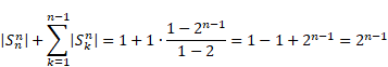If we repeat the same procedure for strings that start with a certain number of consecutive zeroes we will have the same result, . This confirms that in a total there are strings with length n.

Example 4.1. Determine the number of binary strings of length where the first 3 bits are consecutive 1’s.

Solution: According to the formula (1), we have to calculate

Example 4.2. Determine the number of binary strings of length where the first 17 bits are consecutive 1’s.

Solution: According to the formula (1), we have to calculate

We can generate the required strings by recursively invoking the 2NPG(n, k) method (line 3 to 4).

Example 4.3. Determine the number of binary strings of length where at least the first 3 bits are consecutive 1’s.

Solution: According to the formula (1), and the fact that at least the first 3 bits are consecutive 1’s, we have to calculate:

Example 4.4. Determine the number of binary strings of length where the first two bits are 0’s while the third and fourth bits are 1’s.

Solution: We apply the formula (1) for and so we get the number of strings that have at least the first two digits of 1’s. Each of the obtained strings is added by two 0’s at the beginning of the string.

To generate the required strings, we can apply the algorithm for the graph, obtained strings is added by two 0’s at the beginning of the string.

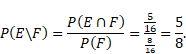
Example 4.5. A bit string of length four is generated at random so that each of the 16 bit strings of length four is equally likely. What is the probability that it contains at least two consecutive 0’s, given that its first bit is a 0? (We assume that 0 bits and 1 bits are equally likely.)

Solution: Let E be the event that a bit string of length four contains at least two consecutive 0s, and let F be the event that the first bit of a bit string of length four is a 0. We can generate the elements of events E and F by applying the graph. Then, the probability that a bit string of length four has at least two consecutive 0 s, given that its first bit is a 0, equals

5. Conclusion

This paper focuses on describing the algorithm of determining the number of binary strings which contain, for a given, exactly runs of 1’s (0’s) of length in all possible binary strings of length , , the graph algorithm has been shown to provide better results to an optimization problem when compared to an equivalent problem related to binary trees.

Detailed knowledge about the distribution of runs in binary strings may be useful in many engineering applications, for example, data compression, bus encoding techniques, computer arithmetic etc. Prior knowledge about the probability of occurrence of runs of 1’s of a given length in a binary string may help us in assessing the merit of a typical run-length encoding scheme. Distribution of runs in binary strings is closely related to the statistics of success runs in n Bernoulli trials with a success probability , and a failure probability of

This paper aims to expand and even further develop the implementation of the algorithm. This will provide many challenges that remain within our ongoing research work.

References

[1] Rosen, K.H. (2003). Discrete Mathematics and Its Applications. New York, NY: Mc Graw Hill.

[2] Underwood, A. (2013). Book Embeddings of Posets. Retrieved from: https://pdfs.semanticscholar.org/2d58/247171aacd351c2871a8389dd216c55aad18.pdf

[3] Cuypers, H. (2007). Discrete Mathematics. Retrieved from: https://pdfs.semanticscholar.org/707d/fd6ea8598d3715934916f73b964a979958c4.pdf

[4] Bigus, P., Tsakovski, S., Simeonov, V., Namiesnik, J., & Tobiszewski, M. (2016). Hasse diagram as a green analytical metrics tool: ranking of methods for benzo[a]pyrene determination in sediment. Analytical and Bioanalytical Chemistry, 408(14), 3833-3841.

[5] Hartman, G., & Green M. (2004). Binary Strings and Graphs. Retrieved from: http://math.arizona.edu/~ura-reports/041/Green.Matthew/Final/bsgf.pdf