An improvement of the sequential algorithm for modeling the chain-like-bodies motion

• BibTex
• RIS
• APA
• Harvard
• IEEE
• MLA
• Vancouver
• Chicago

@article{Bartłomiejczyk_2018,
   doi = {10.17512/jamcm.2018.2.01},
   url = {https://doi.org/10.17512/jamcm.2018.2.01},
   year = 2018,
   publisher = {The Publishing Office of Czestochowa University of Technology},
   volume = {17},
   number = {2},
   pages = {5--16},
   author = {Kamila Bartłomiejczyk},
   title = {An improvement of the sequential algorithm for modeling the chain-like-bodies motion},
   journal = {Journal of Applied Mathematics and Computational Mechanics}
}

TY  - JOUR
DO  - 10.17512/jamcm.2018.2.01
UR  - https://doi.org/10.17512/jamcm.2018.2.01
TI  - An improvement of the sequential algorithm for modeling the chain-like-bodies motion
T2  - Journal of Applied Mathematics and Computational Mechanics
JA  - J Appl Math Comput Mech
AU  - Bartłomiejczyk, Kamila
PY  - 2018
PB  - The Publishing Office of Czestochowa University of Technology
SP  - 5
EP  - 16
IS  - 2
VL  - 17
SN  - 2299-9965
SN  - 2353-0588
ER  - 

Bartłomiejczyk, K. (2018). An improvement of the sequential algorithm for modeling the chain-like-bodies motion. Journal of Applied Mathematics and Computational Mechanics, 17(2), 5-16. doi:10.17512/jamcm.2018.2.01

Bartłomiejczyk, K., 2018. An improvement of the sequential algorithm for modeling the chain-like-bodies motion. Journal of Applied Mathematics and Computational Mechanics, 17(2), pp.5-16. Available at: https://doi.org/10.17512/jamcm.2018.2.01

[1]K. Bartłomiejczyk, "An improvement of the sequential algorithm for modeling the chain-like-bodies motion," Journal of Applied Mathematics and Computational Mechanics, vol. 17, no. 2, pp. 5-16, 2018.

Bartłomiejczyk, Kamila. "An improvement of the sequential algorithm for modeling the chain-like-bodies motion." Journal of Applied Mathematics and Computational Mechanics 17.2 (2018): 5-16. CrossRef. Web.

1. Bartłomiejczyk K. An improvement of the sequential algorithm for modeling the chain-like-bodies motion. Journal of Applied Mathematics and Computational Mechanics. The Publishing Office of Czestochowa University of Technology; 2018;17(2):5-16. Available from: https://doi.org/10.17512/jamcm.2018.2.01

Bartłomiejczyk, Kamila. "An improvement of the sequential algorithm for modeling the chain-like-bodies motion." Journal of Applied Mathematics and Computational Mechanics 17, no. 2 (2018): 5-16. doi:10.17512/jamcm.2018.2.01

AN IMPROVEMENT OF THE SEQUENTIAL ALGORITHM FOR MODELING THE CHAIN-LIKE-BODIES MOTION

Kamila Bartłomiejczyk

Institute of Mathematics, Czestochowa University of Technology
Częstochowa, Poland
kamila.bartlomiejczyk@im.pcz.pl

Received: 6 May 2018; Accepted: 18 June 2018

Abstract. Numerous simulation studies in statistical physics make use of various algorithms that are designed for modeling of the chain-like-body (CLB) motion. In recent years within this group a new sequential algorithm was proposed. The main idea of this new approach to the algorithmization of the CLB motion is based on the incorporation of the tension propagation mechanism into each simulated move. In this paper, improvement of this algorithm by implementation of the direction-preference-mechanism is proposed. This modification enables one to better mimic the real behavior of the CLB. The impact of the new procedure on the simulation process is studied with the help of metamodels that relate to some important characteristics of the CLB motion with the algorithm’s new parameters.

MSC 2010: 68W40, 65C05, 82C41

Keywords: chain-like body, polymer translocation, tension propagation

1. Introduction

The chain-like-body (CLB) consists of small repeating segments/units that are connected with each other so that they form a long chain. CLBs are structures which play an important role in many phenomena in different fields of science. Examples of chain-like-bodies that have attracted much attention recently are polymers and biopolymers [1, 2]. The motion of chain-like bodies is encountered in many physical, chemical, biological and technological processes.

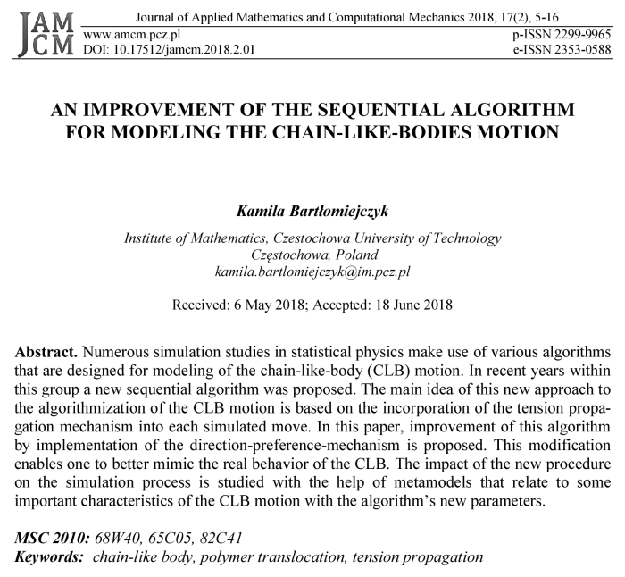
A phenomenon based on the CLB motion which has the greatest interest of researchers is the polymer translocation through the narrow pore of the size comparable with that of a chain segment from one cis-side of a membrane to the other trans-side (see Fig. 1). This phenomenon is ubiquitous in many biological mechanisms in living organisms. For instance, translocation of DNA and RNA across nuclear pores [3, 4], viral injection of DNA into a host cell [5], protein transporting through channels in biological membranes [6], gene transfer between bacteria [7]. The translocation process is investigated via a variety of experiments [1, 8] and theories [1, 8, 9]. However, because of a lot of limitations of experimental studies, this process is also widely studied by simulation experiments [10-12]. It should be mentioned that the translocation of the CLB through the membrane can be done with the presence of an external driving force [1, 2, 11] or without it [8, 13]. Mechanisms which are used as the driving force are e.g. trans-membrane electrical potential, chemical potential gradient, selective adsorption of the chain on one side of membrane (adsorption potential) or solvent selectivity difference.

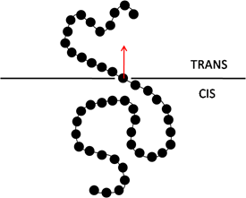
Fig. 1. Schema of the CLB threading through the pore in membrane

A great number of simulation studies use the Monte Carlo to obtain the results, e.g. [8, 10, 13]. Because the MC simulations are addressed to the global (large) scale chain properties, some features of the chain behavior are independent of chemical details. Therefore, these properties can be studied by a simplified ‘coarse-grained’ model. It is a model which associates a group of chemical monomers with a ‘bead’ (effective monomer) to eliminate microscopic degrees of freedom. Such an approach is frequently used in chain-like bodies motion studies, e.g. [14].

In literature, various algorithms that can be used to simulate the CLB motion are presented, e.g. the Fluctuation Bond Method [8, 13, 15] and the pivot algorithm [14]. It can be also found in literature that the researchers developed their own genu- ine algorithms to perform their simulation experiments, e.g. [16, 17]. In this paper, the modification of the sequential algorithm for modeling the chain-like-bodies motion presented in [18] and used for the simulation experiments in [19] is provided. This modification implements the direction-preference-mechanism which enables one to better mimic the real behavior of the CLB. More details about the algorithm and the direction-preference-mechanism is provided in the next section of this paper.

2. Sequential algorithm with built-in tension propagation mechanism

A sequential algorithm for the modeling of the chain-like bodies’ motion with a built-in tension propagation mechanism (SA-CLB) was introduced in [20]. Its detailed description can be found in [18, 19]. In the description of the algorithm, we distinguish steps and moves. A step carries a given single monomer c_i = {x_i,y_i} from one lattice node to another. A single step can randomly transform a randomly chosen monomer into one from a set of its One Step Reachable Nodes (OSRN), i.e. nodes satisfying the condition: , where R_max can be interpreted as the maximum length of a step which can be made in the case where no other (internal) forces and/or restrictions are present. The distance between consecutive segments of the CLB is limited by parameters L_max (maximal length of a step made by any segment; the maximal allowed distance between segments) and L_min (the least possible distance between segments). By making a step, the segment may create a tension in the CLB structure. Particularly, it may happen when the distance between consecutive monomers is greater than some predefined tension constant (T_p). A move of the CLB consists of steps made by consecutive segments as long as the tension in the structure exists. So, the move reflects the tension propagation. If the first step does not create any tension in the CLB structure, then the move may consist of a single step only.

The key feature of this algorithm is the sequentialization of the tension propagation: every move of the CLB is initialized by only one segment. Then the tension propagation through the CLB can be sequentialized into a sequence of steps.

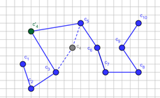
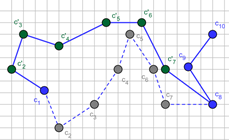
Fig. 2. Exemplary move of the CLB generated by the SA-CLB: a) the first step of the chain is done by segment c₄; c'₄ is a new position of the c₄ , b) steps of the segments caused a chain tension; their new positions are denoted with c'₂¸c'₇ ; Bonds of the final position of the chain are indicated with a solid line. Assumed parameters’ values: R_max = 9, L_min = 2, L_max = 6, T_p = 4

The final CLB position after the move is made may be influenced by various physical laws. In our algorithm these lows can be incorporated into simulation model by a probability distribution defined on the OSRN set. This distribution defines probabilities of different directions and/or lengths of each step. This step probability distribution may also depend on the segment’s coordinates. It will be denoted by SPD. Some features of the environment as well as assumed properties of the CLB itself, may result in the existence of Actually Forbidden Nodes (AFN). For any given moment and for each segment AFN is a subset of OSRN, and, obviously, it may vary in time. The subtraction of OSRN and AFN is called a set of actually accessible nodes: AAN = OSRN-AFN. The distribution SPD truncated to the set AAN is called Actual Step Probability Distribution and denoted ASPD. The next position of a monomer is chosen according to this probability. As usual, finally the move is accepted according to the Metropolis criterion. An exemplary move generated by the algorithm discussed above is illustrated in Figure 2.

3. Movement-direction-preference mechanism

Probability distribution of the actual step (ASPD), in the algorithm described earlier in the previous section, can be dependent on various external laws and on the segments coordinates (and obviously on the SPD which is determined in accordance with the structure and environment parameters’ values). Therefore, each segment can make a step in any direction according to ASPD, and there is no influence of the previous steps of the structure on this direction. However, intuitively it seems to be reasonable to provide a mechanism which makes the consecutive segments’ step direction dependent on the position of the previous segment which has made a step. Thanks to this mechanism, each segment that makes a step can be drug (or pushed) by the neighboring segment in its direction. Thereby, in a new version of the SA-CLB, the ASPD changes during the simulation so that it depends on the position of the segment which has been moved previously. Increase of the probability that the step will be made in the direction of the previous segment which made a step is ensured by the dependence of the ASPD on the values of the cosine function of the angle between vectors or (depending on the direction in which the stress propagation occurs) and , where c_i+1 (c_i–1) is the previous segment which made a step, c_i is the segment which actually makes a step and c_i* is the new position of the c_i segment. The ASPD is multiplied by the value

The symbol α denotes an angle between vectors w₁ and w₂ . M is a parameter which determines how strong the influence is of the previous segment position on the direction of an actually moving segment step. It should be mentioned that when the direction-preference mechanism is disabled. For the purpose of better illustration of the parameter M’s impact on the ASPD and for a more detailed description of the movement-direction preference mechanism, parameter DPI (direction-preference-intensity) is defined. Its value is represented by the following formula:

This parameter indicates how many times greater the chance is that a currently shifting segment will step exactly in the direction of the previously moving segment than the chance that it will move in the opposite direction. To explain and illustrate the influence of DPI on the ASPD, let us study the following example. Let us consider the CLB presented in Figure 3. Segments c₁¸c₄ have already made their steps. Segment c₅ is to make its step as the next one. The empty circles indicate these nodes that are the candidates for a new position of c₅ (i.e. the assumed set of AAN), while the arrows are to indicate exemplary angles which are needed for the calculation of ASPD. The support of the ASPD (and consequently the dimensions of matrix by which it is represented) obviously depend on the algorithm parameters.

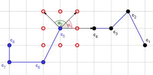
Fig. 3. Illustration of possible position for segment c₅ (empty circles) and exemplary angles (α₁, α₂) which are needed for calculation of ASPD; c₁¸c₄ - segments that already shifts

For the purpose of this example, it is assumed that the matrix that represents the ASPD for c₅ is initially defined as presented in Figure 4.

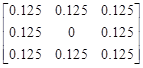
Fig. 4. A matrix which represents the exemplary ASPD for segment c₅ before the application of the movement-direction preference mechanism. The numbers represent the probabilities that the corresponding node (compare Fig. 3) will be occupied by c₅ after the step is made. The number in the center is related to the current position of c₅. Because it is equal to 0, it means that the segment will change its position with probability 1 and its new position will be randomly drawn according the indicated distribution

The collection of numbers indicate the probabilities that the corresponding nodes (represented in Fig. 3 by empty circles) will be occupied by c₅ after the step is made. The number in the center is related to the current position of c₅ . Because it is equal to 0 (generally it does not have to), it indicates that the segment has to change its position (with probability 1). Its new position will be randomly chosen according the distribution represented by the given numbers. In this example, all the candidates are chosen with the same probabilities 0.125. Now, in Figures 5 and 6 the influence of different values of parameters M and DPI on the ASPD is presented. These figures show the impact of movement-direction-preference mechanism on ASPD. In that context, it should be remembered that the previous segment shifts its position to c₄, thus this direction should be preferred now by the algorithm. As it can be seen, for M = 1.1 parameter DPI is equal to 21 and for M = 1.5 it is 5. It means that in case presented in Figure 5, it is 21 times more probable that segment c₅ will shift in the direction of the segment c₄ than that it will shift towards the opposite direction. Obviously, in the case presented in Figure 6 the situation is analogous, only the numbers that represent the probabilities are different due to a different value of the parameter M.

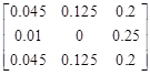
Fig. 5. A matrix which represents the ASPD for segment c₅ after the movement-direction preference mechanism application with DPI = 21 and M = 1.1

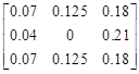
Fig. 6. A matrix which represents the ASPD for segment c₅ after the movement-direction preference mechanism application with DPI = 5 and M = 1.5

In the above figures it can be noticed that increment of the value of the DPI results in increment of disproportions in the values of the probabilities assigned to opposite directions. One can see that the bigger the DPI, the bigger the chance is that the currently shifting segment will make a step towards the previously moving one.

As it was mentioned earlier, a symbol α in formula (1) denotes an angle between vectors w₁ and w₂ . Obviously the greater the value of , the higher probabil- ity of making the step in the direction indicated be the vector w₂ . Exemplary angles between these vectors are presented in Figure 7. The segments indicated by black dots (c₆ , c₇ , c₈) are segments which have already made steps and their positions cannot be changed. The next step is to be made by the segment c₅ . Two different new positions of the segment c₅ are illustrated in Figure 7. They are denoted by c'₅ . Thus, and . In the first case (a), the angle between vectors w₁ and w₂ (the α₁) is an obtuse angle, while in the second case (b) the angle between these vectors (the α₂) is the acute angle. Because of the fact that and (and therefore ), the new position of c₅ presented in Figure 7b is more probable than position presented in Figure 7a.

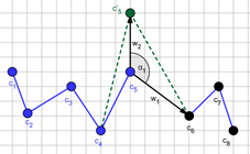
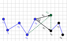
Fig. 7. Exemplary angles which determined changes of ASPD: a) an obtuse angle (α₁), b) an acute angle (α₂). Segments which have already made steps are denoted with c₆ , c₇ and c₈ , segments c₁¸c₅ are before their steps. c'₅ is a possible new position of segment c₅

4. Simulation experiment and metamodels

The algorithm which is discussed above is implemented in the simulation environment designed in Wolfram Mathematica (version 10.4). The simulation experiment was performed with the following values of algorithm parameters: , , , . The forced translo- cation process of the chain through the pore in the membrane was simulated. Therefore, an additional parameter P responsible for an existence of driving force was also used. This parameter has an influence on the ASPD. Its value causes that the probability of a step in the direction of the trans-side of the barrier (for each moving segment) is P times more than in another direction. The values of parameter P in performed simulation experiment were from the range [2,5]. Following the literature, it is assumed that initially the first monomer of the chain is in the pore, see e.g. [21]. Such an assumption allows one to neglect the way of the pore in membrane reaching. The initial position of the relaxed chain is randomly chosen from the set of different positions. The translocation time τ (the passage time) is defined as the time which is needed to translocate all monomers through the pore on the other side of membrane. When the last monomer crosses the membrane, the translocation time is saved and the simulation is finished. Therefore, the translocation can be treated as successful only if the chain is translocated from the initial side (cis) to the other side (trans) of membrane. The simulations were performed for two chain lengths: N = 30 and N = 60. On the basis of the results obtained from the simulations, two metamodels relating the passage time and algorithm parameters are built and presented here. The aim of this modeling is twofold. First it is interesting to verify whether the introduced parameters of the algorithm have impact on this passage time. If so, then the models could help the researcher in appropriate adjustment of these parameters to make the algorithm mimic the underlying real phenomenon (passage time in this case) as well as possible.

The first model built on the basis of the simulation experiment result is the linear model. This shape of the regression function is often used for modeling physical and engineering phenomena because it is able to capture the real statistical relationship between the observable input and output, especially when the values of parame- ters vary in small ranges. The metamodel in the following form is built:

where Z is a random variable (disturbance).

With the help of the regression analysis tools the following linear regression function has been estimated for N = 30:

The estimates of the regression coefficients , of metamodel (4) obtained for N = 30 are as in Table 1. The statistical characteristics of these estimates are presented in Table 2.

Table 1

The values of the regression coefficients of the linear model given by eq. (4) for N = 30

Table 2

The values of statistical characteristics of the regression coefficients of the linear model given by eq. (4) for N = 30

In Table 1, it can be seen that all explanatory variables have a significance level less than , while usually is assumed to be small enough to justify the statement that the corresponding variables are significant in the model. The coefficient of determination of the model (4) is equal to . It tells one that about 49% of the total variation of the passage time is due to changes in the parameters’ values. Intuitive interpretation, often adopted in such a case by practitioners, is that the behavior of the dependent variable is explained in 49% by the explanatory variables. The rest of variation is a result of the impact of other (not included in the model) variables or - as in this case - is a realization of a purely random process. It can be seen in Table 1 that increasing the parameters R_max , T_p , P and DPI causes a decrease of the τ. It confirms the expectations based on the intuition and, consequently, it supports correctness of the incorporation of the new parameters into the SA-CLB algorithm. It should be mentioned that such a linear regression model is also built for chain length N = 60. The estimation of this model parameters is qualitatively the same as in the linear model for N = 30.

The second metamodel built on the basis of the simulation results is the log-log (loglinear) model. It is useful for the analysis of the elasticity of the passage time with respect to the algorithm parameters. The following loglinear metamodel has been built:

The estimates g_i of the regression coefficients γ_i , i = 0,…,5 which have been obtained for N = 30 are presented in Table 3. Table 4 contains the statistical characteristics of these estimates.

Table 3

The values of the regression coefficients of the loglinear model given by eq. (5) for N = 30

Tables 1-3 confirm the conclusions obtained from the linear model, i.e. the increase of parameters R_max , T_p , P and DPI causes the decrease of τ whereas the increase of the L_max causes the increase of τ. Moreover, as it can be seen in Table 4, all explanatory variables appear to be significant because their significance level is much lower than the usually assumed . The coefficient of determination is equal to R² = 0.5570 which is comparable with this obtained in previously described metamodel. The values of the regression coefficients reflect the percentage change in τ as a response for a given unit-percentage change in a given explanatory variable. Therefore, e.g. when the value of parameter P goes up by 1 percent on average (and the other parameters remain the same), the value of τ goes down by about 0.35%. It should be mentioned that the estimation of model (5) parameters is qualitatively the same in the loglinear model for N = 60.

Table 4

The values of statistical characteristics of the regression coefficients of the loglinear model by eq. (5) for N = 30

It is worth emphasizing that from the statistical point of view, both presented models are correct. An additional test performed to choose a best possible regression function (PE test) results in the conclusion that all the functions can be considered as proper ones, at least in the range of observed (in the simulations) parameter values.

7. Conclusions

This paper discusses the movement-direction-preference mechanism which is incorporated to the sequential algorithm for the modeling of the chain-like bodies’ motion (SA-CLB). This mechanism makes the consecutive segments’ step direction dependent on the position of the previous segment which has made a step. A simulation study of the CLB translocation through the pore is performed. On the basis of the results obtained in a simulation experiment, two metamodels are built. They allow one to relate the passage time τ with the algorithm parameters: R_max , L_max , T_p , P and DPI.

Both presented models confirm that all considered algorithm-parameters have an impact on the passage time. In particular, the parameter DPI implemented in the movement-direction-preference mechanism has an influence on τ. Thus, it confirms that the modification of the SA-CLB algorithm is reasonable. It can be seen that the influence of the algorithm parameters on the passage time is as follows: the greater the parameters R_max , T_p , P and DPI the less is the passage time and the greater the parameter L_max the greater is the passage time.

It should be mentioned that the linear model (4) is better for quantitative analysis of the influence of the particular parameter on the passage time. On the other hand, the loglinear model (5) is better choice in the case of the elasticity study.

Metamodels building can be helpful for the researchers in appropriate adjustment of parameters so the performance of the SA-CLB algorithm would mimic/reflect the specific physical phenomenon. Therefore, it allows one to plan the simulation experiment that reflects the real phenomenon.

References

[1] Dubbeldam, J.L.A., Rostiashvili, V.G., Milchev, A., & Vilgis, T.A. (2012). Forced translocation of polymer: Dynamical scaling versus molecular dynamics simulation. Physical Review E, 85, 041801.

[2] Huopaniemi, I., & Luo, K. (2006). Langevin dynamics simulations of polymer translocation through nanopores. The Journal of Chemical Physics, 125, 124901.

[3] Liang, L., Shen, J-W., Zhang, Z., & Wang, Q. (2017). DNA sequencing by two-dimensional materials: As theoretical modeling meets experiments. Biosensors and Bioelectronics, 89, 280-292.

[4] Panja, D., Barkema, G.T., & van Leeuwen, J.M.J. (2016). Dynamics of a double-stranded DNA segment in a shear flow, arXiv: 1603.05227v1 [cond-mat.soft].

[5] Gundersen-Rindal, D. (2012). Integration of Polydnavirus DNA into Host Cellular Genomic DNA, In: Parasitoid Viruses. Symbionts and Pathogens, 99-113.

[6] Wickner, W., & Schekman, R. (2005). Protein translocation across biological membranes. Science, 310, 1452-6.

[7] Miller, T.V. (1998). Bacterial Gene Swapping in Nature. Scientific American.

[8] Luo, K., Ala-Nissila, T., & Ying, S.C. (2006). Polymer translocation through a nanopore: A two-dimensional Monte Carlo Study. The Journal of Chemical Physics, 124(3), 034714.

[9] Lubensky, D.K., & Nelson, D.R. (1999). Driven polymer translocation through a narrow pore. Biophysical Journal, 77, 1824-1838.

[10] Abdolvahab, R.H. (2006). Investigating binding particles distribution effects on polymer translocation through nanopore. Physics Letters A, 380, 1023-1030.

[11] Sarabadani, J., Ghosh, B., Chaudhury, S., & Ala-Nissila, T. (2017). Dynamics of end-pulled polymer translocation through a nanopore, arXiv:1708.09184 [cond-mat.soft].

[12] Żurek, S., Kośmider, M., Drzewiński, A., & van Leeuwen, J.M.J. (2012). Translocation of polymers in a lattice model. The European Phys. J. E: Soft Matter and Biological Physics, 35, 47.

[13] Chatelain, C., Kantor, Y., & Kardar, M. (2008). Probability distributions for polymer translocation. Physical Review E, 78, 021129.

[14] D’Adamo, G., Pelissetto, A., & Pierleoni, C. (2012). Polymers as compressible soft spheres. arXiv: 1205.5654v1, cond-mat.soft.

[15] Kolli, H.B., & Murthy, K.P.N. (2012). Phase transition in a bond fluctuating lattice polymer, arXiv: 1204.2691v2 [cond-mat.soft].

[16] Gauthier, M.G., & Slater, G.W. (2008). A Monte Carlo algorithm to study polymer translocation through nanopores. I. Theory and numerical approach. The Journal of Chemical Physics, 128, 065103.

[17] Gauthier, M.G. & Slater, G.W. (2008). A Monte Carlo algorithm to study polymer translocation through nanopores. II. Scaling laws. The Journal of Chemical Physics, 128, 205103.

[18] Grzybowski, A.Z., & Domanski, Z. (2011). A sequential algorithm for modeling random movements of chain-like structures. Scientific Research of the Institute of Mathematics and Computer Science, 10(1), 5-10.

[19] Grzybowski, A.Z., Domański, Z., & Bartłomiejczyk, K. (2013). Algorithmization and simulation of the chain-like structures’ dynamics-interrelations between movement characteristics. Acta Eletrotechnica et Informatica, 13(4).

[20] Grzybowski, A.Z., & Domański, Z. (2013). A sequential algorithm with built in tension-propagation mechanism for modeling the chain-like bodies dynamics, http://arxiv.org/pdf/ 1312.4206v1.pdf.

[21] Yu, W., Ma, Y., & Luo, K. (2012). Translocation of stiff polymers through a nanopore driven by binding particles. The Journal of Chemical Physics, 137, 244905.