Spectral-homotopy analysis of MHD non-orthogonal stagnation point flow of a nanofluid
Sarkhosh S. Chaharborj
,Abbas Moameni
Journal of Applied Mathematics and Computational Mechanics |
 Download Full Text |
 View in HTML format |
 Export citation |
@article{Chaharborj_2018,
   doi = {10.17512/jamcm.2018.1.02},
   url = {https://doi.org/10.17512/jamcm.2018.1.02},
   year = 2018,
   publisher = {The Publishing Office of Czestochowa University of Technology},
   volume = {17},
   number = {1},
   pages = {15--28},
   author = {Sarkhosh S. Chaharborj and  Abbas Moameni},
   title = {Spectral-homotopy analysis of MHD non-orthogonal stagnation point flow of a nanofluid},
   journal = {Journal of Applied Mathematics and Computational Mechanics}
}
TY - JOUR DO - 10.17512/jamcm.2018.1.02 UR - https://doi.org/10.17512/jamcm.2018.1.02 TI - Spectral-homotopy analysis of MHD non-orthogonal stagnation point flow of a nanofluid T2 - Journal of Applied Mathematics and Computational Mechanics JA - J Appl Math Comput Mech AU - Chaharborj, Sarkhosh S. AU - Moameni, Abbas PY - 2018 PB - The Publishing Office of Czestochowa University of Technology SP - 15 EP - 28 IS - 1 VL - 17 SN - 2299-9965 SN - 2353-0588 ER -
Chaharborj, S., & Moameni, A. (2018). Spectral-homotopy analysis of MHD non-orthogonal stagnation point flow of a nanofluid. Journal of Applied Mathematics and Computational Mechanics, 17(1), 15-28. doi:10.17512/jamcm.2018.1.02
Chaharborj, S. & Moameni, A., 2018. Spectral-homotopy analysis of MHD non-orthogonal stagnation point flow of a nanofluid. Journal of Applied Mathematics and Computational Mechanics, 17(1), pp.15-28. Available at: https://doi.org/10.17512/jamcm.2018.1.02
[1]S. Chaharborj and A. Moameni, "Spectral-homotopy analysis of MHD non-orthogonal stagnation point flow of a nanofluid," Journal of Applied Mathematics and Computational Mechanics, vol. 17, no. 1, pp. 15-28, 2018.
Chaharborj, Sarkhosh S., and Abbas Moameni. "Spectral-homotopy analysis of MHD non-orthogonal stagnation point flow of a nanofluid." Journal of Applied Mathematics and Computational Mechanics 17.1 (2018): 15-28. CrossRef. Web.
1. Chaharborj S, Moameni A. Spectral-homotopy analysis of MHD non-orthogonal stagnation point flow of a nanofluid. Journal of Applied Mathematics and Computational Mechanics. The Publishing Office of Czestochowa University of Technology; 2018;17(1):15-28. Available from: https://doi.org/10.17512/jamcm.2018.1.02
Chaharborj, Sarkhosh S., and Abbas Moameni. "Spectral-homotopy analysis of MHD non-orthogonal stagnation point flow of a nanofluid." Journal of Applied Mathematics and Computational Mechanics 17, no. 1 (2018): 15-28. doi:10.17512/jamcm.2018.1.02
SPECTRAL-HOMOTOPY ANALYSIS OF MHD NON-ORTHOGONAL STAGNATION POINT FLOW OF A NANOFLUID
Sarkhosh S. Chaharborj 1,2, Abbas Moameni 1
1 School of Mathematics and Statistics, Carleton University, Ottawa,
K1S 5B6, Canada
2 Department of Mathematics, Islamic Azad University, Bushehr
Branch, Bushehr, Iran
saman.seddighi@carleton.ca, momeni@math.carleton.ca
Received: 14 May 2017;
Accepted: 24 January 2018
Abstract. In this article, we investigate the theoretical study of the magnetohy-drodynamic (MHD) non-orthogonal stagnation point flow of a nanofluid towards a stretching. The partial differential equations that model the problem are reduced to ordinary differential equations which are then solved analytically using the improved Spectral Homotopy Analysis Method (SHAM). Comparisons of our results from SHAM and numerical solutions show that this method is a capable tool for solving this type of linear and nonlinear problems semi-analytically.
MSC 2010: 34B15, 34K07, 34K28
Keywords: nanofluid, MHD stagnation flow, stretching sheet, SHAM
1. Introduction
The boundary layer flow problems have various applications in the fluid mechanics. Namely, the classical two-point nonlinear boundary value Blasius problem which models viscous fluid flow over a semi-infinite flat plate, nonlinear Falkner-Skan equation and magnetohydro dynamic (MHD) boundary layer flow.
Most researchers have used the semi-analytical and numerical methods such as the Runge-Kutta methods [1], finite difference methods [2], finite element methods [3] and spectral methods [4] to solve this type of equations. In recent years, for solving nonlinear differential equations, several analytical and semi-analytical methods have been established such as the variational iteration method [5, 6], Adomian decomposition method [7], differential transform method [8], homotopy analysis method (HAM) [9-13], and the spectral-homotopy analysis (SHAM) [14, 15] and more recently, the successive linearization method [16, 17].
All analytical and semi-analytical methods mostly focus on the single and independent linear and nonlinear equations of the boundary layer flow problems. In this paper, we present an improved spectral-homotopy analysis method to solve the system of boundary layer problems. The considered system contains the nonlinear boundary differential equations governed from partial differential equations of magnetohydrodynamic (MHD) non-orthogonal stagnation point flow of a nanofluid towards a stretching.
2. Formulation of the problem
We investigate the steady two-dimensional
stagnation point flow of a second grade nanofluid over a stretching surface [18, 19]. Two equal and opposite forces are applied along the z-axis so that
the surface is stretched keeping the origin fixed, as shown in Figure 1. We further assume that the surface has temperature ![]() and the fluid has
uniform ambient temperature
and the fluid has
uniform ambient temperature ![]() (here
(here ![]() ). The flow is
subjected to the combined effect of thermal radiation and a transverse magnetic
field of strength
). The flow is
subjected to the combined effect of thermal radiation and a transverse magnetic
field of strength ![]() , which is assumed to be applied in the positive
, which is assumed to be applied in the positive ![]() direction, normal to the surface. The induced magnetic field is
also assumed negligible compared to the applied magnetic field, so it can be
neglected. It is further assumed that the base fluid and the suspended
nanoparticles are in thermal equilibrium. It is chosen that the coordinate
system
direction, normal to the surface. The induced magnetic field is
also assumed negligible compared to the applied magnetic field, so it can be
neglected. It is further assumed that the base fluid and the suspended
nanoparticles are in thermal equilibrium. It is chosen that the coordinate
system ![]() -axis is along the
stretching sheet and
-axis is along the
stretching sheet and ![]() -axis is normal to the
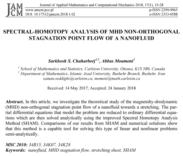
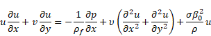
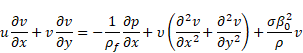
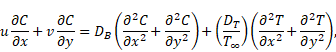
sheet. Under the above assumptions, the governing equation of the conservation of mass, momentum, energy and nanoparticles
fraction in the presence of a magnetic field and thermal radiation past
a stretching sheet can be expressed as,
-axis is normal to the
sheet. Under the above assumptions, the governing equation of the conservation of mass, momentum, energy and nanoparticles
fraction in the presence of a magnetic field and thermal radiation past
a stretching sheet can be expressed as,
 |
 |
 |
 |
on ![]() .
.
Here ![]() and
and ![]() are the velocity components in the x and y
directions.
are the velocity components in the x and y
directions. ![]() and k are the local temperature of the fluid, nano-particle fraction,
kinematic
viscosity, density, electrical conductivity, and permeability of the saturated
porous medium parameters, respectively.
and k are the local temperature of the fluid, nano-particle fraction,
kinematic
viscosity, density, electrical conductivity, and permeability of the saturated
porous medium parameters, respectively. ![]() is the thermal
diffusivity,
is the thermal
diffusivity, ![]() is
the Brownian motion coefficient, in general the thermal diffusion coefficient
is
the Brownian motion coefficient, in general the thermal diffusion coefficient ![]() is a function of temperature and concentration, which complicates the
description of thermophoresis and
is a function of temperature and concentration, which complicates the
description of thermophoresis and ![]() is the ratio of
effective heat capacity of the nanoparticle material to heat capacity of the
fluid and
is the ratio of
effective heat capacity of the nanoparticle material to heat capacity of the
fluid and ![]() is the density of nano-
fluid at constant pressure. The boundary conditions are,
is the density of nano-
fluid at constant pressure. The boundary conditions are,
| (1) |
Where ![]() and
and ![]() , are positive constants with the dimension of (time)–1 indicating
potential flow and linear shear flow parallel to the streamwise direction
(shear stress
, are positive constants with the dimension of (time)–1 indicating
potential flow and linear shear flow parallel to the streamwise direction
(shear stress ![]() ) contributions into
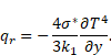
the oblique flow, respectively. Radiative heat flux
) contributions into
the oblique flow, respectively. Radiative heat flux ![]() in governing boundary layer equation of energy is
approximated by Rosseland
approximation, which gives,
in governing boundary layer equation of energy is
approximated by Rosseland
approximation, which gives,
 |
It is assumed that the temperature difference
within the flow is so small that ![]() can be expressed as a linear function of
can be expressed as a linear function of ![]() . This can be obtained by expanding
. This can be obtained by expanding ![]() in a Taylor series about
in a Taylor series about ![]() and neglecting the
higher order terms will results
and neglecting the
higher order terms will results ![]() .
Heat is transferred by forced convection, which
involves the only normal component of flow field. Introducing the following
dimensionless quantities, the mathematical analysis of the problem is
simplified by using similarity transformations.
.
Heat is transferred by forced convection, which
involves the only normal component of flow field. Introducing the following
dimensionless quantities, the mathematical analysis of the problem is
simplified by using similarity transformations.
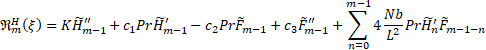
According to the presented similarity transformations as shown in [18, 19], the above systems can be converted to the following ordinary differential equations along with the corresponding boundary conditions,
| (2) |
| (3) |
|
|
|
| (5) |
on ![]() and subject to the
boundary conditions,
and subject to the
boundary conditions,
| (6) |
| (7) |
where, ![]() and
and ![]() are positive constants and
are positive constants and ![]() is striking angle,
is striking angle, ![]() is the magnetic
number,
is the magnetic
number, ![]() is the Prandtl number,
is the Prandtl number,
![]() is thermal radiation
effect,
is thermal radiation
effect, ![]() is the thermophoresis
parameter,
is the thermophoresis
parameter, ![]() is the Lewis number.
is the Lewis number.
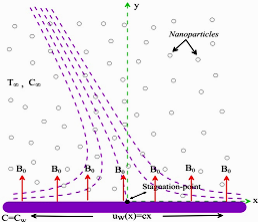
Fig. 1. Geometry of problem
3. The spectral homotopy analysis method
At the beginning, for transferring the domain
of the problem from ![]() to
to ![]() , the domain truncation method has been utilized. The computational
domain
, the domain truncation method has been utilized. The computational
domain ![]() where
where ![]() is a fixed length can be used to approximate the domain
is a fixed length can be used to approximate the domain ![]() . Here,
. Here, ![]() is taken to be larger
than the thickness of the boundary layer [15]. The simple
algebraic mapping for transferring the interval
is taken to be larger
than the thickness of the boundary layer [15]. The simple
algebraic mapping for transferring the interval ![]() to the Chebyshev domain
to the Chebyshev domain ![]() is as follows,
is as follows,
|
|
|
For convenience, the boundary conditions have been made homogeneous by applying the transformations as,
| (9) |
where, ![]() ,
, ![]() ,
, ![]() and
and ![]() are chosen so as to
satisfy the boundary conditions (6) and (7) as,
are chosen so as to
satisfy the boundary conditions (6) and (7) as,
| (10) |
Substituting Eqs. (10) into Eqs. (2)-(7) yields that,
|
|
|
||||
|
|
|
||||
|
|
|
||||
|
|
|
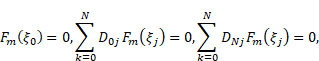
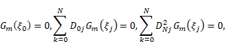
with the boundary conditions,
| (15) |
where the
coefficients ![]() in Eq. (11) are defined by,
in Eq. (11) are defined by,
![]()
![]()
![]()
![]()
![]() and the coefficients
and the coefficients ![]() in Eq. (12) appear as following:
in Eq. (12) appear as following:
![]()
![]()
![]()
![]()
![]()
![]()
and here are the coefficients ![]() and
and ![]() in Eqs. (13) and (14) respectively,
in Eqs. (13) and (14) respectively,
![]()
![]()
![]()
![]()
![]()
![]()
By solving the linear parts of Eqs. (2) up to (5), we can obtain the initial solutions,
|
|
|
||||
|
|
|
| (18) |
|
|
|
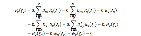
subject to the boundary conditions,
| (20) |
The Chebyshev pseudo-spectral method has been
used to solve Eqs. (16) up to (19). The unknown
functions ![]() and
and![]() are aproximated as
truncated series of Chebyshev polynomials as follows,
are aproximated as
truncated series of Chebyshev polynomials as follows,
| (21) |
where ![]() and
and ![]() are the Chebyshev polynomials with
coefficients
are the Chebyshev polynomials with
coefficients ![]()
![]() ,
, ![]() and
and ![]() respectively;
respectively; ![]() ,
, ![]() are Gauss-Lobatto
collocation points defined as,
are Gauss-Lobatto
collocation points defined as, ![]()
Derivatives of the functions ![]() ,
, ![]() ,
, ![]() and
and ![]() at the collocations
points are defined as,
at the collocations
points are defined as,
|
|
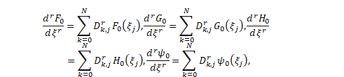
where
![]() is the order of differentiation and
is the order of differentiation and ![]() is the Chebyshev
spectral differential matrix with the entries as,
is the Chebyshev
spectral differential matrix with the entries as,
![]()
![]()
with
![]() is defined as follows,
is defined as follows,
![]()
substituting
Eqs. (21) into Eqs. (16)-(19) yields, ![]() subject to the
boundary conditions,
subject to the
boundary conditions,
|
|
where,
|
|
![]()
![]()
![]()
![]()
![]()
![]()
The superscript T
denotes the transpose, “diag” is a diagonal matrix
and I is an identity matrix of size ![]() . The values of
. The values of ![]() are obtained from the
equation,
are obtained from the
equation, ![]() which
which ![]() is the initial
approximation for the solution of Eqs. (11)-(14) by the
SHPM.
The 0-th order deformation equations are given by,
is the initial
approximation for the solution of Eqs. (11)-(14) by the
SHPM.
The 0-th order deformation equations are given by,
![]()
![]()
![]()
![]()
with,
![]() .
.
here H is the nonzero convergence controlling auxiliary parameter; L and N are linear and nonlinear operators, respectively, defined as,
![]()
![]()
![]()
![]()
![]()
![]()
![]()
![]()
The ![]() -th order deformation
equations are given by,
-th order deformation
equations are given by,
| (25) |
subject to the boundary conditions,
| (26) |
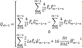
![]()
where:
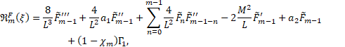
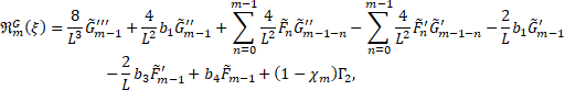
![]()

| (27) |
Applying the Chebyshev pseudospectral transformation to Eqs. (25)-(27) gives,
| (28) |
subject to the boundary conditions:
| (29) |
where ![]() are defined in Eq. (24)
and
are defined in Eq. (24)
and
![]()
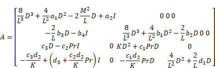
Boundary conditions (29) are implemented in matrix A on the left side of (28)
in rows ![]() ,
, ![]() ,
, ![]() ,
, ![]() and
and ![]() , respectively. Matrix
, respectively. Matrix ![]() in the right-hand side of Eq. (28),
in the right-hand side of Eq. (28), ![]() and
and ![]() have corresponding
rows and all columns equal to zero. This recursive formula when
have corresponding
rows and all columns equal to zero. This recursive formula when ![]() , can be written as follows,
, can be written as follows,
| (30) |
Therefore, the higher-order approximation ![]() for
for ![]() has been obtained by starting from the initial approximation.
has been obtained by starting from the initial approximation.
4. Optimization of convergence-control parameters based on the square residual errors
From Eqs. (27), error functions can be defined as follows:
| (31) |
In what follows, we are going to find the
optimal values of ![]() ,
, ![]() ,
, ![]() and
and ![]() , by using the
convergence-control for various values of order
, by using the
convergence-control for various values of order ![]() will find. The square residual error (SRE) method can help us to
optimize the convergence-control
parameters as follows:
will find. The square residual error (SRE) method can help us to
optimize the convergence-control
parameters as follows:
| (32) |
| (33) |
where ![]() ,
, ![]() ,
, ![]() and
and ![]() are the
are the ![]() th-order SHAM approximations of the functions
th-order SHAM approximations of the functions ![]() ,
, ![]() ,
, ![]() and
and ![]() , respectively.
Obviously, when
, respectively.
Obviously, when ![]() then we will have
then we will have ![]() ,
, ![]() ,
, ![]() and
and ![]() that correspond to
convergent series solutions of SHAM. The points at which the gradient of square
residual error functions presented in Eqs. (32) and
(33) with respect to convergence-control parameters vanish, are precisely
the optimal values of
that correspond to
convergent series solutions of SHAM. The points at which the gradient of square
residual error functions presented in Eqs. (32) and
(33) with respect to convergence-control parameters vanish, are precisely
the optimal values of ![]() ,
, ![]() ,
, ![]() and
and ![]() for
for ![]() th-order SHAM approximation as follows:
th-order SHAM approximation as follows:
|
|
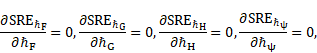
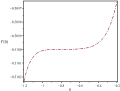
Figure 2 presents the
optimal values ![]() and the optimal square
residual errors
in the
and the optimal square
residual errors
in the ![]()
![]() at different values of
at different values of ![]() . This figure shows that the optimal values of
. This figure shows that the optimal values of ![]() is approximately
between –1 and –0.4. By choosing
is approximately
between –1 and –0.4. By choosing ![]() from this optimal
interval, the results obtained from SHAM will have good accuracy. Table 1 presents the optimal values of
from this optimal
interval, the results obtained from SHAM will have good accuracy. Table 1 presents the optimal values of ![]() ,
, ![]() ,
, ![]() and
and ![]()
![]() and optimal values of the square residual error at a different order
of
and optimal values of the square residual error at a different order
of ![]() in the
in the ![]() . Table 1 is showing that with
increasing the order of approximation
. Table 1 is showing that with
increasing the order of approximation ![]() , the square residual
error will decrease. To obtain the results of Table 1, Matlab R2015b software
has been used.
, the square residual
error will decrease. To obtain the results of Table 1, Matlab R2015b software
has been used.
|
|
|
|
Fig. 2. Optimal |
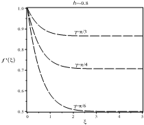
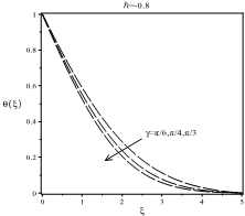
Fig. 3. Influence of |
|
|
|
|
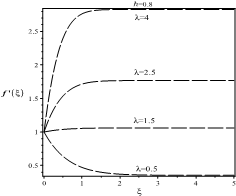
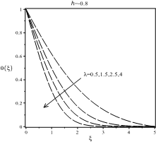
Fig. 4. Influence of |
Fig. 5. Influence of |
|
|
|
|
Fig. 6.
Influence of |
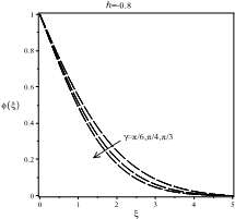
Fig. 7.
Influence of |
|
|
Table 1 The optimal values |
||||||||||||||||||||||||||||||||||||
|
|||||||||||||||||||||||||||||||||||||
|
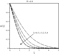
Fig. 8.
Influence of |
5. Results and discussion
Figures 3, 5 and 7 present the influence of ![]() on
on ![]() and, temperature and
concen-
tration profiles when
and, temperature and
concen-
tration profiles when ![]() and
and ![]()
![]() . As shown, by
decreasing the values of
. As shown, by
decreasing the values of ![]() appeared in the
initial conditions
appeared in the
initial conditions ![]() and
and ![]() from
from ![]() to
to ![]() the profile
the profile ![]() is decreasing and both
temperature and concentration profiles
is decreasing and both
temperature and concentration profiles ![]() and
and ![]() are increasing. The results indicate that the curves reduce with a
negative slope for
are increasing. The results indicate that the curves reduce with a
negative slope for ![]() . Figure 3 is showing
that with decreasing the striking angle
. Figure 3 is showing
that with decreasing the striking angle ![]() at a fixed value of
at a fixed value of ![]() , heat
transfer velocity will decrease. Figure 5 indicates that with decreasing the
striking angle at a fixed value of
, heat
transfer velocity will decrease. Figure 5 indicates that with decreasing the
striking angle at a fixed value of ![]() , temperature will
increase. Figure 7 is showing that with
decreasing the striking angle at a fixed value of
, temperature will
increase. Figure 7 is showing that with
decreasing the striking angle at a fixed value of ![]() , heat transfer concentration will increase.
, heat transfer concentration will increase.
Figures 4, 6 and 8 are showing the influence of ![]() on
on ![]() and, temperature and
concentration profiles when
and, temperature and
concentration profiles when ![]() and
and ![]() . Note that, by increasing the values of
. Note that, by increasing the values of ![]() appeared in the initial condition
appeared in the initial condition ![]() form 0.5 to 4 the
profile
form 0.5 to 4 the
profile ![]() is increasing and both
temperature and concentration profiles
is increasing and both
temperature and concentration profiles ![]() and
and ![]() are decreasing. Figures 4 indicate,
however, that they have positive slopes for
are decreasing. Figures 4 indicate,
however, that they have positive slopes for ![]() , and the curves reduce with a negative slope for
, and the curves reduce with a negative slope for ![]() . Figure 4 is showing
that with increasing the velocity parameter
. Figure 4 is showing
that with increasing the velocity parameter ![]() at a fixed value of
at a fixed value of ![]() , heat transfer
velocity will increase. Figure 6 indicates that with increasing the velocity
parameter at a fixed value of
, heat transfer
velocity will increase. Figure 6 indicates that with increasing the velocity
parameter at a fixed value of ![]() , temperature will
increase. Figure 8 is showing that with increasing the velocity parameter at a
fixed value of
, temperature will
increase. Figure 8 is showing that with increasing the velocity parameter at a
fixed value of ![]() , heat transfer
concentration will increase.
, heat transfer
concentration will increase.
In order to test the accuracy of the present
results, we have compared the results for skin friction coefficient ![]() with those reported by
Lok et al. [20]. This
comparison is presented in Table 2. It is noticed that this comparison shows
an excellent agreement, so that we are confident that the present results are
accurate. Table 2 shows a comparison of the
results
with those reported by
Lok et al. [20]. This
comparison is presented in Table 2. It is noticed that this comparison shows
an excellent agreement, so that we are confident that the present results are
accurate. Table 2 shows a comparison of the
results ![]() for for
for for ![]() at different values of
at different values of ![]() and
and ![]() . Results of this table indicate that with increasing parameter
. Results of this table indicate that with increasing parameter ![]() from 0.2 to 3.0, for any values of parameter
from 0.2 to 3.0, for any values of parameter ![]() ,
, ![]() is increasing. As
seen, by increasing
is increasing. As
seen, by increasing ![]() from
from ![]() to
to ![]() , the function
, the function ![]() is increasing with a
high speed. To obtain the results of Table 2, Matlab R2015b software has been
used.
is increasing with a
high speed. To obtain the results of Table 2, Matlab R2015b software has been
used.
Table 2
Comparison of the results for ![]() for
for ![]() at different values of
at different values of
![]() and
and ![]() .
With
.
With ![]() and
and ![]()
|
|
|
|||||||
|
|
|
|
|
|||||
|
Present |
Lok et al. [20] |
Present |
Lok et al. [20] |
Present |
Lok et al. [20] |
Present |
Lok et al. [20] |
|
|
0.2 |
–0.987616 |
–0.987032 |
–0.950564 |
–0.950424 |
–0.933744 |
–0.933660 |
–0.918165 |
–0.918110 |
|
0.5 |
–0.956437 |
–0.956268 |
–0.806205 |
–0.806205 |
–0.734439 |
–0.734444 |
–0.667265 |
–0.667271 |
|
1.0 |
–0.879693 |
–0.879674 |
–0.424309 |
–0.424315 |
–0.205021 |
–0.205025 |
– |
– |
|
2.0 |
–0.648607 |
–0.648613 |
0.738447 |
0.738474 |
1.400957 |
1.401023 |
2.017503 |
2.017615 |
|
3.0 |
–0.331931 |
–0.331937 |
2.313007 |
2.313144 |
3.566349 |
3.566614 |
4.729282 |
4.729694 |
Conclusion
We have investigated the modified spectral
homotopy analysis method (SHAM) for solving a complicated nonlinear dynamical
system in the MHD non-orthogonal stagnation point flow of a nanofluid towards a
stretching. Numerical results show the effectiveness of our proposed method for
solving complicated linear and non-linear dynamical systems in the heat
transfer and heat flow problems. The results indicate
that they have positive slopes for ![]() , and the curves reduce
with
a negative slope for
, and the curves reduce
with
a negative slope for ![]() . The optimal interval
for
. The optimal interval
for ![]() is between –1 and
–0.4. The results for skin friction coefficient
is between –1 and
–0.4. The results for skin friction coefficient ![]() from our presented
method with
from our presented
method with ![]() and
and ![]() have been compared with those reported by Lok et al.
at references [20]. This comparison shows an excellent agreement, so that we
are confident that the present results are accurate.
have been compared with those reported by Lok et al.
at references [20]. This comparison shows an excellent agreement, so that we
are confident that the present results are accurate.
References
[1] Chaharborj, S.S., Kiai, S.S., Bakar, M.A., Ziaeian, I., & Fudziah, I. (2012). New impulsional potential for a paul ion trap. International Journal of Mass Spectrometry, 309, 63-69.
[2] Nayak, I., Nayak, A.K., & Padhy, S. (2016). Implicit fnite difference solution for the magneto- hydro-dynamic unsteady free convective flow and heat transfer of a third-grade fluid past a porous vertical plate. International Journal of Mathematical Modelling and Numerical Optimisation, 7(1), 4-19.
[3] John, V. (2016). Finite Element Methods for Incompressible Flow Problems. Berlin: Erscheint demnchst bei Springer.
[4] Chen, S., & Wang, Y. (2016). A rational spectral collocation method for third-order singularly perturbed problems. Journal of Computational and Applied Mathematics, 307, 93-105.
[5] Moameni, A. (2011). Non-convex self-dual lagrangians: New variational principles of symmetric boundary value problems. Journal of Functional Analysis, 260(9), 2674-2715.
[6] Wazwaz, A.M. (2016). Solving systems of fourth-order emden-fowler type equations by the variational iteration method. Chemical Engineering Communications, 203(8), 1081-1092.
[7] Hosseini, S., Babolian, E., & Abbasbandy, S. (2016). A new algorithm for solving van der pol equation based on piecewise spectral adomian decomposition method. International Journal of Industrial Mathematics, 8(3), 177-184.
[8] Fidanoglu, M., Komurgoz, G., & Ozkol, I. (2016). Heat transfer analysis of fins with spine geometry using differential transform method. International Journal of Mechanical Engineering and Robotics Research, 5(1), 67-71.
[9] Shahlaei-Far, S., Nabarrete, A., & Balthazar, J.M. (2016). Homotopy analysis of a forced nonlinear beam model with quadratic and cubic nonlinearities. Journal of Theoretical and Applied Mechanics, 54(4), 1219-1230.
[10] Semary, M.S., & Hassan, H.N. (2016). The homotopy analysis method for q-difference equations. Ain Shams Engineering Journal, DOI http://dx.doi.Org/10.1016/j.asej.2016.02.005.
[11] Hayat, T., Mumtaz, M., Shafiq, A., & Alsaedi, A. (2017). Stratified magnetohydrodynamic flow of tangent hyperbolic nanofluid induced by inclined sheet. Applied Mathematics and Mechanics, 38(2), 271-288.
[12] Zhu, J., Wang, S., Zheng, L., & Zhang, X. (2017). Heat transfer of nanofluids considering nanoparticle migration and second-order slip velocity. Applied Mathematics and Mechanics, 38(1), 125-136.
[13] Zhao, Q., Xu, H., Tao, L., Raees, A., & Sun, Q. (2016). Three-dimensional free bio-convection of nanofluid near stagnation point on general curved isothermal surface. Applied Mathematics and Mechanics, 37(4), 417-432
[14] Motsa, S.S., Marewo, G.T., Sibanda, P., & Shateyi, S. (2011). An improved spectral homotopy analysis method for solving boundary layer problems. Boundary Value Problems, 2011(1), 3-11.
[15] Rashidi, M.M., Rostami, B., Freidoonimehr, N., & Abbasbandy, S. (2014). Free convective heat and mass transfer for MHD fluid flow over a permeable vertical stretching sheet in the presence of the radiation and buoyancy effects. Ain Shams Engineering Journal, 5(3), 901-912.
[16] Bhatti, M.M., Shahid, A., & Rashidi, M.M. (2016). Numerical simulation of fluid flow over a shrinking porous sheet by Successive linearization method. Alexandria Engineering Journal, 55(1), 51-56.
[17] Ahmed, M.A.M., Mohammed, M.E., & Khidir, A.A. (2015). On linearization method to MHD boundary layer convective heat transfer with low pressure gradient. Propulsion and Power Research, 4(2), 105-113.
[18] Rashidi, M.M., Abelman, S., & Mehr, N.F. (2013). Entropy generation in steady MHD flow due to a rotating porous disk in a nanofluid. International Journal of Heat and Mass Transfer, 62, 515-525.
[19] Rashidi, M.M., Ali, M., Freidoonimehr, N., & Nazari, F. (2013). Parametric analysis and optimization of entropy generation in unsteady MHD flow over a stretching rotating disk using artificial neural network and particle swarm optimization algorithm. Energy, 55, 497-510.
[20] Lok, Y.Y., Amin, N., & Pop, I. (2006). Non-orthogonal stagnation point flow towards a stretching sheet. International Journal of Non-Linear Mechanics, 41(4), 622-627.