Analytical and numerical solution of the heat conduction problem in the rod

• BibTex
• RIS
• APA
• Harvard
• IEEE
• MLA
• Vancouver
• Chicago

@article{Węgrzyn-Skrzypczak_2017,
   doi = {10.17512/jamcm.2017.4.08},
   url = {https://doi.org/10.17512/jamcm.2017.4.08},
   year = 2017,
   publisher = {The Publishing Office of Czestochowa University of Technology},
   volume = {16},
   number = {4},
   pages = {79--86},
   author = {Ewa Węgrzyn-Skrzypczak and  Tomasz Skrzypczak},
   title = {Analytical and numerical solution of the heat conduction problem in the rod},
   journal = {Journal of Applied Mathematics and Computational Mechanics}
}

TY  - JOUR
DO  - 10.17512/jamcm.2017.4.08
UR  - https://doi.org/10.17512/jamcm.2017.4.08
TI  - Analytical and numerical solution of the heat conduction problem in the rod
T2  - Journal of Applied Mathematics and Computational Mechanics
JA  - J Appl Math Comput Mech
AU  - Węgrzyn-Skrzypczak, Ewa
AU  - Skrzypczak, Tomasz
PY  - 2017
PB  - The Publishing Office of Czestochowa University of Technology
SP  - 79
EP  - 86
IS  - 4
VL  - 16
SN  - 2299-9965
SN  - 2353-0588
ER  - 

Węgrzyn-Skrzypczak, E., & Skrzypczak, T. (2017). Analytical and numerical solution of the heat conduction problem in the rod. Journal of Applied Mathematics and Computational Mechanics, 16(4), 79-86. doi:10.17512/jamcm.2017.4.08

Węgrzyn-Skrzypczak, E. & Skrzypczak, T., 2017. Analytical and numerical solution of the heat conduction problem in the rod. Journal of Applied Mathematics and Computational Mechanics, 16(4), pp.79-86. Available at: https://doi.org/10.17512/jamcm.2017.4.08

[1]E. Węgrzyn-Skrzypczak and T. Skrzypczak, "Analytical and numerical solution of the heat conduction problem in the rod," Journal of Applied Mathematics and Computational Mechanics, vol. 16, no. 4, pp. 79-86, 2017.

Węgrzyn-Skrzypczak, Ewa, and Tomasz Skrzypczak. "Analytical and numerical solution of the heat conduction problem in the rod." Journal of Applied Mathematics and Computational Mechanics 16.4 (2017): 79-86. CrossRef. Web.

1. Węgrzyn-Skrzypczak E, Skrzypczak T. Analytical and numerical solution of the heat conduction problem in the rod. Journal of Applied Mathematics and Computational Mechanics. The Publishing Office of Czestochowa University of Technology; 2017;16(4):79-86. Available from: https://doi.org/10.17512/jamcm.2017.4.08

Węgrzyn-Skrzypczak, Ewa, and Tomasz Skrzypczak. "Analytical and numerical solution of the heat conduction problem in the rod." Journal of Applied Mathematics and Computational Mechanics 16, no. 4 (2017): 79-86. doi:10.17512/jamcm.2017.4.08

ANALYTICAL AND NUMERICAL SOLUTION OF THE HEAT CONDUCTION PROBLEM IN THE ROD

Ewa Węgrzyn-Skrzypczak ¹, Tomasz Skrzypczak ²

¹ Institute of Mathematics, Czestochowa University of Technology
Czestochowa, Poland
² Institute of Mechanics and Machine Design Fundamentals Czestochowa University of Technology,
Czestochowa, Poland
ewa.skrzypczak@im.pcz.pl, t.skrzypczak@imipkm.pcz.pl

Received: 20 October 2017; Accepted: 16 November 2017

Abstract. In this paper, the results of analytical and numerical solution of the problem of heat transport in the rod of finite length are presented. The analytical solution is obtained with the use of the Fourier series. The numerical model of the problem is based on the Finite Element Method (FEM). In addition, to check the compatibility of both solutions, distributions of the temperature for selected time moments are compared and discussed.

MSC 2010: 35K05,35K51, 65M60

Keywords: heat conduction equation, Fourier’s method, Finite Element Method

1. Introduction

During the investigation of the physical or technical processes, one strives to find the rules governing the process and derive the analytical expressions describing the functional dependencies between the variables. In physics most of the laws of nature can be written in the form of differential equations [1].

In order to find the solution of differential equations, the analytical methods are used, which allow one to find a solution in the form of equations determining the sought quantity expressed by elementary functions. Such a form of solution makes it possible to obtain any results of the boundary value problem by means of mathe-matical analysis tools [1]. Unfortunately, in many cases, the complexity of the considered problem (e.g. the irregularity of the examined area or the complexity of the partial differential equations) makes it impossible to obtain the analytical solutions. The only alternative in this situation is to use one of many numerical methods (e.g. finite difference method, finite element method [2, 3]) to find the approximate solution of the problem [4-8].

However, the results of the numerical method require verification. The best way to validate the results obtained with the use of the numerical method is the com- parison with the analytical solution of the considered problem. In the case of good agreement of compared analytical and numerical solutions one has the proof that the numerical method is mathematically correct.

2. Formulation of the problem

The heat conduction problem in the finite rod of length lying on the x-axis is considered. The ends of the rod are located at the points and respec- tively. The end A of the rod is thermally insulated, while the opposite end B is kept at constant temperature . It is assumed that the temperature on the cross-sectional area of the rod is uniform due to its small dimensions. At the time , the initial temperature distribution along the rod is defined by the function , where . The temperature in the rod is the function of position and time [1, 9]. The scheme of the problem is presented in Figure 1.

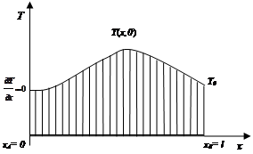
Fig. 1. Scheme of the problem

The transient heat transfer in the rod is described by the equation of heat conduction [3, 10, 11] in the form shown below:

(1)

The coefficient a² is described by the following relation:

(2)

where: - temperature, - time, - the coefficient of thermal conductivity, - specific heat, - density.

Equation (1) is supplemented by the boundary conditions of the first and second kind [3, 10, 11]:

,

(3)

(4)

The initial condition is also defined:

(5)

3. Analytical solution

In order to determine the analytical solution of equation (1) with the boundary conditions (3), (4), the new function is introduced [10]:

(6)

Consequently, the boundary conditions (3), (4) take the form:

(7)

(8)

while the initial condition (5) is presented below:

(9)

Now, equation (1) can be written in the following form:

(10)

The solution of equation (10) is obtained with the use of the Fourier method [10] in the form of the function of two variables (11), where the first depends on while the second is the function of :

(11)

By substituting relation (11) into equation (10) and by dividing it by the following relation is obtained:

(12)

where the value of is constant. Further equations are obtained from equation (12):

(13)

(14)

By substituting the solutions of the equations (13), (14) into (11) and by using the conditions (7), (8) the following equation is obtained [10]:

(15)

where is constant. Using condition (9) and assuming that meets the condi- tions of expansion in the Fourier series and additionally , the following analytical solution of equation (1) can be written in the form shown below:

(16)

where: for .

4. Numerical solution

To obtain a numerical solution of equation (1), the finite element method is used [2, 3]. Equation (1) is multiplied by the weighting function and integrated over the length of the rod:

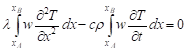(17)

Using integration by parts (18), (19) the first term in equation (17) may be written in the form (20).

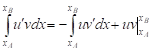(18)

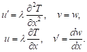(19)

(20)

Heat flux at the points and is defined as follows:

(21)

Finally, the weak form of the equation of heat conduction takes the following form:

(22)

Equation (22) is discretized over the space with the use of the Galerkin method where the weighting functions are the same as the shape functions N of the finite elements. Then the implicit time integration scheme is used to obtain a global set of equations. The final form of the global FEM equation is shown below [9]:

(23)

where: is the global thermal conductivity matrix, - global heat capacity matrix, - right hand side vector, - time step, - time level.

5. Examples of calculation

The solutions of equation (1) are obtained using the boundary conditions (3), (4), the initial condition (5) and the material properties presented in Table 1.

Table 1

Parameters used in calculations

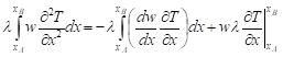
In Figures 2 and 3, the results of the analytical solution obtained with the use of the Fourier series and numerical model of the problem based on the FEM are shown.

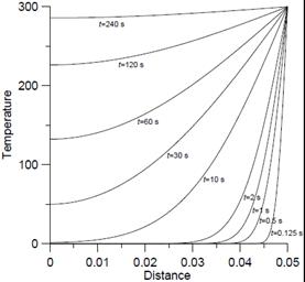
Fig. 2. Analytical solution for selected time moments

Fig. 3. Numerical solution for selected time moments

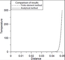
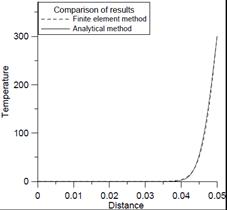
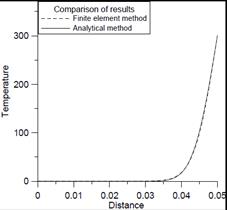
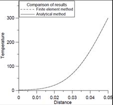
Also, to check compatibility of both solutions, in Figure 4 temperature distri- butions obtained as a result of both solutions for selected time moments are presented.

a) b)

c) d)

e) f)

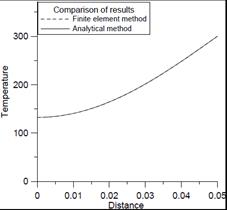
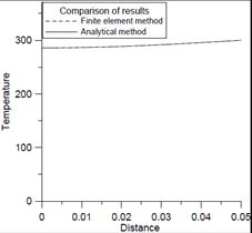
Fig. 4. Temperature distributions obtained as a result of analytical and numerical solutions for 0.125 s (a), 0.5 s (b), 1 s (c), 10 s (d), 60 s (e), 240 s (f)

6. Conclusions

The analysis of obtained results confirms the good compatibility of both models, which proves their correctness. Changes of temperature distribution due to time are clearly visible. The differences in the temperature distributions gradually decrease as time passes and vanish almost completely at the end of the process. The numerical solution is obtained for the mesh containing 101 nodes, while only 100 consecutive terms are used to obtain an analytical solution. Increasing the number of nodes in the first case and the number of terms in the second do not improve the results significantly.

Built models can be modified in a relatively simple way to solve two-dimens-ional and three-dimensional heat conduction problems. In this case, the analytical method will be limited to simple geometry, but in the case of a numerical model such constraints do not exist.

References

[1] Tichonow A.N., Samarski A.A., Równania fizyki matematycznej, PWN, Warszawa 1963.

[2] Majchrzak E., Mochnacki B., Metody numeryczne. Podstawy teoretyczne, aspekty praktyczne i algorytmy, Wydawnictwo Politechniki Śląskiej, Gliwice 1994.

[3] Mochnacki B., Suchy J., Modelowanie i symulacja krzepnięcia odlewów, WN PWN, Warszawa 1993.

[4] Zienkiewicz O.C., Taylor R.L., The finite element method, Volume 3: Fluid dynamics, Butterworth and Hienemann, 2000.

[5] Bokota A., Kulawik A., Model and numerical analysis of hardening process phenomena for medium-carbon steel, Archives of Metallurgy and Materials 2007, 52, 337-346.

[6] Skrzypczak T., Węgrzyn-Skrzypczak E., Mathematical and numerical model of solidification proces of pure metals, International Journal of Heat and Mass Transfer 2012, 555, 4276-4284.

[7] Mendakiewicz J., Identification of solidification proces parameters, Computer Assisted Mechanics and Engineering Sciences (CAMES) 2010, 17(1), 59-73.

[8] Mochnacki B., Suchy S.J., Numerical methods in computations of foundary processes, Polish Foundrymen’s Technical Association, Krakow 1995.

[9] Zaporożec G.I., Metody rozwiązywania zadań z analizy matematycznej, WNT, Warszawa 1967.

[10] Fichtenholz G.M., Rachunek różniczkowy i całkowy, WN PWN, Warszawa 1999.

[11] Longa W., Krzepnięcie odlewów w formach piaskowych, Wydawnictwo „Śląsk”, Katowice 1973.