A design of an optimal shape of domain described by NURBS curves using the topological derivative and boundary element method
Katarzyna Freus
,Sebastian Freus
Journal of Applied Mathematics and Computational Mechanics |
 Download Full Text |
 View in HTML format |
 Export citation |
@article{Freus_2017,
   doi = {10.17512/jamcm.2017.2.06},
   url = {https://doi.org/10.17512/jamcm.2017.2.06},
   year = 2017,
   publisher = {The Publishing Office of Czestochowa University of Technology},
   volume = {16},
   number = {2},
   pages = {67--76},
   author = {Katarzyna Freus and  Sebastian Freus},
   title = {A design of an optimal shape of domain described by NURBS curves using the topological derivative and boundary element method},
   journal = {Journal of Applied Mathematics and Computational Mechanics}
}
TY - JOUR DO - 10.17512/jamcm.2017.2.06 UR - https://doi.org/10.17512/jamcm.2017.2.06 TI - A design of an optimal shape of domain described by NURBS curves using the topological derivative and boundary element method T2 - Journal of Applied Mathematics and Computational Mechanics JA - J Appl Math Comput Mech AU - Freus, Katarzyna AU - Freus, Sebastian PY - 2017 PB - The Publishing Office of Czestochowa University of Technology SP - 67 EP - 76 IS - 2 VL - 16 SN - 2299-9965 SN - 2353-0588 ER -
Freus, K., & Freus, S. (2017). A design of an optimal shape of domain described by NURBS curves using the topological derivative and boundary element method. Journal of Applied Mathematics and Computational Mechanics, 16(2), 67-76. doi:10.17512/jamcm.2017.2.06
Freus, K. & Freus, S., 2017. A design of an optimal shape of domain described by NURBS curves using the topological derivative and boundary element method. Journal of Applied Mathematics and Computational Mechanics, 16(2), pp.67-76. Available at: https://doi.org/10.17512/jamcm.2017.2.06
[1]K. Freus and S. Freus, "A design of an optimal shape of domain described by NURBS curves using the topological derivative and boundary element method," Journal of Applied Mathematics and Computational Mechanics, vol. 16, no. 2, pp. 67-76, 2017.
Freus, Katarzyna, and Sebastian Freus. "A design of an optimal shape of domain described by NURBS curves using the topological derivative and boundary element method." Journal of Applied Mathematics and Computational Mechanics 16.2 (2017): 67-76. CrossRef. Web.
1. Freus K, Freus S. A design of an optimal shape of domain described by NURBS curves using the topological derivative and boundary element method. Journal of Applied Mathematics and Computational Mechanics. The Publishing Office of Czestochowa University of Technology; 2017;16(2):67-76. Available from: https://doi.org/10.17512/jamcm.2017.2.06
Freus, Katarzyna, and Sebastian Freus. "A design of an optimal shape of domain described by NURBS curves using the topological derivative and boundary element method." Journal of Applied Mathematics and Computational Mechanics 16, no. 2 (2017): 67-76. doi:10.17512/jamcm.2017.2.06
A DESIGN OF AN OPTIMAL SHAPE OF DOMAIN DESCRIBED BY NURBS CURVES USING THE TOPOLOGICAL DERIVATIVE AND BOUNDARY ELEMENT METHOD
Katarzyna Freus1, Sebastian Freus2
1Institute
of Mathematics, Czestochowa University of Technology, Poland
2 Institute of Computer and Information Science, Czestochowa
University of Technology
Czestochowa, Poland
katarzyna.freus@im.pcz.pl, sebastian.freus@icis.pcz.pl
Received: 30 April 2017; accepted: 17 May 2017
Abstract. The aim of this paper is to create an optimal shape of the 2D domain that is described by the Non-Uniform Rational B-Splines (NURBS) curves. This work presents a method based on the topological derivative for the Laplace equation that determines the sensitivity of a given cost function to the change of its topology. As a numerical approach, the boundary element method is considered. To check the effectiveness of the proposed approach, the example of computations was carried out.
MSC 2010: 35J25, 65N38, 49K10, 49Q10, 53A04
Keywords: Laplace equation, boundary element method, topological derivative, NURBS curves
1. Introduction
Topological optimization is a mathematical method that allows one to find an optimal material layout of a domain, such that a cost function gives its optimum value after optimization under given constraints. Material is removed by creating a small hole that appears in the optimization process. The topological derivative (DT) indicates the position in the domain of interest where a hole should be formed. Wherever DT is low enough, a hole is created. In the opening, the Neumann condition is taken into account. The topological-shape sensitivity method is utilized as a procedure to calculate the topological derivative taking the total potential energy as a cost function [1-4]. The boundary of the domain is described by the NURBS curves which are commonly used for representing and designing a shape in numerical implementation. In order to determine the temperature field of the domain considered, the boundary element method (BEM) is used in its direct version. In this paper, firstly a review of the BEM and the NURBS curves are presented. After that, the topological derivative for the Laplace equation is introduced and the numerical results are shown. Finally, conclusions are expressed.
2. Boundary element method
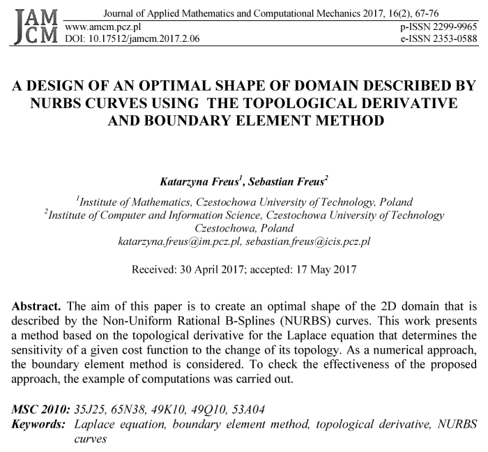
The domain W bounded by contour Γ is taken into account. The Laplace equation supplemented by the boundary condition is the following [4, 5]
 (1)
(1)
where x = (x1, x2) are the spatial coordinates, λ [W/mK] is the thermal conductivity, T (x) denotes the temperature, ∂T /∂n is the normal derivative, n = [cosa1, cosa2] is the normal outward vector. Tb and qb are known as the boundary temperature and heat flux, respectively. T¥ is the ambient temperature and α [W/m2 K] is the heat transfer coefficient. The boundary integral equation for problem (1) is the following
![]() (2)
(2)
where ![]() is the coefficient connected with the local shape of a boundary,
x is the
observation point and
is the coefficient connected with the local shape of a boundary,
x is the
observation point and ![]() is the heat flux.
is the heat flux. ![]() and
and ![]() are
the following
are
the following
![]() ,
, ![]() (3)
(3)
where r indicates the distance between x = (x1, x2) and x = (x1, x2)
![]() (4)
(4)
while
![]() (5)
(5)
nx, ny are the directional cosines of the normal outward vector n.
Using the linear boundary elements, Equation (2) can be given in the form
| | (6) |
Considering the known boundary condition, Eq. (6) can be written
![]() (7)
(7)
where A is the main matrix, X is the unknown vector and B is the free terms vector. Equation (7) ensures the determination of the missing boundary conditions.
3. NURBS curves
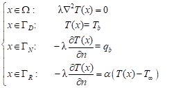
In the numerical example, we take into account the domain Ω where the segments of the boundary are described by the NURBS curves so, in this part of paper, we present the main information about these curves. A n-th degree NURBS curve is as follows
 | (8) |
where wj are the weights, Pj are the control points forming a control polygon and Nj,n (t) are the B-spline basis functions
| (9) |
prescribed for the set of nodes
| (10) |
at the same time the values a and b appear n +1 times. It should be mentioned that the number of control points equals r +1 and corresponds to the number of nonzero basis functions. Details about the NURBS curves can be found in [6].
4. Topological derivative
In this work, the topological derivative for
the Laplace equation is considered. In the inside of the original domain W, a small hole
of radius ![]() is created. The idea of the topological
derivative is based on determining the sensitivity of a given cost function (total
potential energy) when the size of this hole is changed. The local value of the
DT is defined as follows [1-4]
is created. The idea of the topological
derivative is based on determining the sensitivity of a given cost function (total
potential energy) when the size of this hole is changed. The local value of the
DT is defined as follows [1-4]
![]() (11)
(11)
where ![]() and
and ![]() are
the cost functions calculated for the original W and the new domain
are
the cost functions calculated for the original W and the new domain ![]() , respectively, and f is a
regularizing function. There
are several papers in the area of the DT for the steady state heat transfer. In this work, we adopt the definition called the topological - shape
sensitivity method proposed in [1], which is based on the following formula
, respectively, and f is a
regularizing function. There
are several papers in the area of the DT for the steady state heat transfer. In this work, we adopt the definition called the topological - shape
sensitivity method proposed in [1], which is based on the following formula
![]() (12)
(12)
where ![]() is a small perturbation on the radius of
the hole.
is a small perturbation on the radius of
the hole.
5. Problem formulation
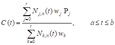
Let ![]() be the domain with a small hole. The Laplace equation
supplemented by the boundary conditions is taken into account [1-4]
be the domain with a small hole. The Laplace equation
supplemented by the boundary conditions is taken into account [1-4]
 (13)
(13)
where on the holes He created via DT, the Neumann boundary condition is prescribed. Problem (13) can be
written in the variational form with a test function ![]() Find
Find ![]() such that
such that
![]() (14)
(14)
For the perturbed configuration, expression (14) is the following
 (15) (15) |
Using the total potential energy [1], the
cost function ![]() for problem (13) has the form
for problem (13) has the form
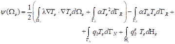 (16)
(16)
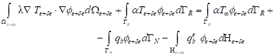
The optimization problem can be expressed as the minimization of equation (16) with the variational formulation (Eq. (14) and (15)) as constraints. All these equations are used to obtain topological derivative (12). After some mathematical manipulations, the final expression for the topological derivative is the following
![]() (17)
(17)
It is important to mention that T is the solution of the original problem (without a hole). Details of the calculation of DT are described in [1-3].
In this work, the
gradient ![]() is obtained by differentiating the integral equation
is obtained by differentiating the integral equation
![]() (18)
(18)
with respect to the internal points, so
![]() (19)
(19)
where ![]() and
and ![]() are given by expressions (3).
are given by expressions (3).
In order to obtain an optimal shape of the domain, we perform the iterative procedure that is carried out in some steps. First, the initial domain described by the NURBS curves and the stopping criterion are provided. Then, using the BEM, the temperature field is obtained. Next, the topological derivative at the boundary nodes is calculated by means of expressions (17). The point with the lowest absolute value of DT is chosen. On the selected point a hexagonal hole is created (Fig. 1).
It is assumed that the side length of a
regular hexagon is approximately equal to the length of the
boundary element (i.e. the arithmetic average of the
length of all the boundary elements). So, a radius r of the hole can be
changed by increasing or decreasing the numbers of the boundary and internal
nodes. Generally the radius is a fraction ![]() of a
dimension of the original domain (this means
of a
dimension of the original domain (this means ![]() where
d = min(height,width)) [3].
where
d = min(height,width)) [3].
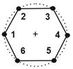
Fig. 1. Hexagonal hole
On the hole the Neumann condition is prescribed. Finally, the boundary of the domain is rebuilt. All the previous steps are repeated until a given stop criterion is obtained. The material volume is checked and removed after each iteration until an expected value is obtained. The elimination process of material is halted when
![]() (20)
(20)
where b presents a determined percentage of material to be eliminated.
6. Numerical example and results
This section presents the solution of a problem defined by (13). It is assumed that l = 30 W/mK. Figure 2 illustrates dimensions of the domain considered while Figure 3 shows the position of control points: P0 = (0, 0), P1 = (0.02, 0), P2 = (0.02, 0.015), P3 = (0.035, 0.015), P4 = (0.05, 0.015), P5 = (0.05, 0), P6 = (0.104, 0), P7 = (0.104, 0.011), P8 = (0.115, 0.011), P9 = (0.126, 0.011), P10 = (0.126, 0), P11 = (0.15, 0), P12 = (0.15, 0.075), P13 = (0.075, 0.075), P14 = (0, 0.075).
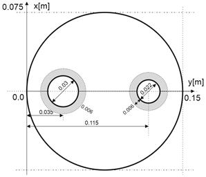
Fig. 2. Domain considered
Since the original domain is symmetrical, only half of the domain will be taken into account in further examination. The boundary of the region is represented by the NURBS curves as follows (see Figs. 3 and 4):
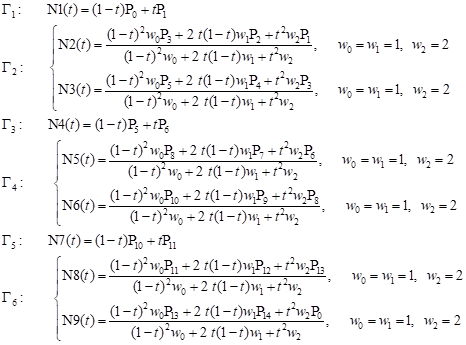
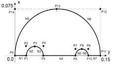
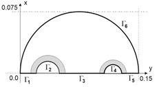
Fig. 3. Position of control points Fig. 4. Segments of boundary
The gray area (see Figures 2 and 4) will not
be perturbed (this is the structural part of the problem). On the top of the
domain (G6), the Robin condition is
considered where the heat transfer coefficient is α = 10 W/ (m2K) and the ambient
temperature is T∞ = 20°C. On the boundary ![]() the temperature Tb =
500°C is
accepted while on
the temperature Tb =
500°C is
accepted while on ![]() , Tb = 200°C
is given.
, Tb = 200°C
is given.
On the remaining parts of the boundary the Neumann condition qb = 0 is prescribed. The initial boundary was divided into 90 linear boundary elements and the grid of 298 internal nodes was used.
Figure 5 illustrates the temperature distribution
while Figure 6 shows the topological
derivative calculated in the first iteration (k = 1). Figure 7 presents the domain after the first iteration. In the opening, ![]() is assumed. Holes with
is assumed. Holes with
![]() 0.002 were
used and during each iteration 3% of
material was eliminated. The iterative procedure was stopped when 60% of
material from the initial domain was removed.
The final result is presented in Figure 8.
0.002 were
used and during each iteration 3% of
material was eliminated. The iterative procedure was stopped when 60% of
material from the initial domain was removed.
The final result is presented in Figure 8.
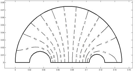
Fig. 5. Temperature distribution
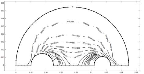
Fig. 6. Topological derivative at k = 1
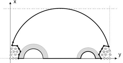
Fig. 7. Domain after the first iteration
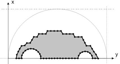
Fig. 8. Final result
7. Conclusions
In the present work, the boundary element method and the topological derivative are used to obtain an optimal shape of the domain described by NURBS curves. The topological-shape sensitivity method gives information about the position where the opening can be inserted. The appropriate criterion is used to stop creating holes. After applying the iterative process, an optimal shape of the domain is found. To inspect the correctness of the method, the example of computation was conducted. The proposed approach confirms an effective the BEM coupled with the NURBS curves and the DT implementation for the design of an optimal topology of the domain considered applied in the heat transfer process modelling.
References
[1] Navotny A.A., Feijoo R.A., Taroco E., Padra C., Topological-shape sensitivity analysis, Comput. Methods Appl. Mech. Eng. 2003, 192, 803-829.
[2] Marczak R.J., Topology optimization and boundary elements - a preliminary implementation for linear heat transfer, Engineering Analysis with Boundary Elements 2007, 31, 793-802.
[3] Anflor C.T.M., Marczak R.J., Topological sensitivity analysis for two-dimensional heat transfer problems using the Boundary Element Method, Optimization of Structures and Components Advanced Structured Materials 2013, 43, 11-33.
[4] Anflor C., Marczak R.J., A boundary element approach for shape and topology design in orthotropic heat transfer problems, Mecanica Computacional vol. XXVII, 2473-2486, San Luis, Argentina, 10-13 Noviembre 2008.
[5] Brebbia C.A., Dominguez J., Boundary Elements, An Introductory Course, CMP, McGraw-Hill Book Company, London 1992.
[6] Majchrzak E., Boundary Element Method in Heat Transfer, Publ. of the Techn. Univ. of Czest., Czestochowa 2001 (in Polish).
[7] Piegl L., Tiller W., The NURBS Book, Springer, 1995.