Numerical solutions of a steady 2-D incompressible flow in a rectangular domain with wall slip boundary conditions using the finite volume method
Vusala Ambethkar
,Mohit Kumar Srivastava
Journal of Applied Mathematics and Computational Mechanics |
 Download Full Text |
 View in HTML format |
 Export citation |
@article{Ambethkar_2017,
   doi = {10.17512/jamcm.2017.2.01},
   url = {https://doi.org/10.17512/jamcm.2017.2.01},
   year = 2017,
   publisher = {The Publishing Office of Czestochowa University of Technology},
   volume = {16},
   number = {2},
   pages = {5--16},
   author = {Vusala Ambethkar and  Mohit Kumar Srivastava},
   title = {Numerical solutions of a steady 2-D incompressible flow in a rectangular domain with wall slip boundary conditions using the finite volume method},
   journal = {Journal of Applied Mathematics and Computational Mechanics}
}
TY - JOUR DO - 10.17512/jamcm.2017.2.01 UR - https://doi.org/10.17512/jamcm.2017.2.01 TI - Numerical solutions of a steady 2-D incompressible flow in a rectangular domain with wall slip boundary conditions using the finite volume method T2 - Journal of Applied Mathematics and Computational Mechanics JA - J Appl Math Comput Mech AU - Ambethkar, Vusala AU - Srivastava, Mohit Kumar PY - 2017 PB - The Publishing Office of Czestochowa University of Technology SP - 5 EP - 16 IS - 2 VL - 16 SN - 2299-9965 SN - 2353-0588 ER -
Ambethkar, V., & Srivastava, M. (2017). Numerical solutions of a steady 2-D incompressible flow in a rectangular domain with wall slip boundary conditions using the finite volume method. Journal of Applied Mathematics and Computational Mechanics, 16(2), 5-16. doi:10.17512/jamcm.2017.2.01
Ambethkar, V. & Srivastava, M., 2017. Numerical solutions of a steady 2-D incompressible flow in a rectangular domain with wall slip boundary conditions using the finite volume method. Journal of Applied Mathematics and Computational Mechanics, 16(2), pp.5-16. Available at: https://doi.org/10.17512/jamcm.2017.2.01
[1]V. Ambethkar and M. Srivastava, "Numerical solutions of a steady 2-D incompressible flow in a rectangular domain with wall slip boundary conditions using the finite volume method," Journal of Applied Mathematics and Computational Mechanics, vol. 16, no. 2, pp. 5-16, 2017.
Ambethkar, Vusala, and Mohit Kumar Srivastava. "Numerical solutions of a steady 2-D incompressible flow in a rectangular domain with wall slip boundary conditions using the finite volume method." Journal of Applied Mathematics and Computational Mechanics 16.2 (2017): 5-16. CrossRef. Web.
1. Ambethkar V, Srivastava M. Numerical solutions of a steady 2-D incompressible flow in a rectangular domain with wall slip boundary conditions using the finite volume method. Journal of Applied Mathematics and Computational Mechanics. The Publishing Office of Czestochowa University of Technology; 2017;16(2):5-16. Available from: https://doi.org/10.17512/jamcm.2017.2.01
Ambethkar, Vusala, and Mohit Kumar Srivastava. "Numerical solutions of a steady 2-D incompressible flow in a rectangular domain with wall slip boundary conditions using the finite volume method." Journal of Applied Mathematics and Computational Mechanics 16, no. 2 (2017): 5-16. doi:10.17512/jamcm.2017.2.01
NUMERICAL SOLUTIONS OF A STEADY 2-D INCOMPRESSIBLE FLOW IN A RECTANGULAR DOMAIN WITH WALL SLIP BOUNDARY CONDITIONS USING THE FINITE VOLUME METHOD
Vusala Ambethkar1, Mohit Kumar Srivastava2
1Department of Mathematics, Faculty of Mathematical Sciences,
University of Delhi, India
2Delhi College of Arts & Commerce, University of Delhi, Delhi, India
vambethkar@maths.du.ac.in, vambethkar@gmail.com, srivastava264@gmail.com
Received: 26 January 2017; accepted: 17 May 2017
Abstract. In this study, a finite volume method (FVM) is suitably used for solving the problem of a fully coupled fluid flow in a rectangular domain with slip boundary conditions. Numerical solutions for the flow variables, viz. velocity, and pressure have been computed. The FVM, with an upwind scheme, has been implemented to discretize the governing equations of the present problem. The well known SIMPLE algorithm is employed for pressure-velocity coupling. This was executed with the aid of a computer program developed and run in a C-compiler. Computations have been performed for unknown variables with Reynolds numbers (Re) = 50, 100, 250, 500, 750 and 1000. The behavior of steady-state solutions of velocity and pressure of the fluid along horizontal and vertical through geometric center of the rectangular domain have been illustrated. We observed that, with the increase of the Reynolds number, the absolute value of velocity components decreases whereas the pressure value increases.
MSC 2010: 35Q30, 65M08, 65N08, 74S10, 76D05, 76M12
Keywords: finite volume method, numerical solutions, pressure, Reynolds number, SIMPLE algorithm, staggered grid, u-velocity, v-velocity
1. Introduction
The problem of steady incompressible fluid flow has been the subject of intensive numerical computations in recent years due to its significant applications in many scientific and engineering practices. Fluid flows play an important role in various equipment and processes. The steady 2-D incompressible viscous flow is a complex problem of great practical significance. The study of fluid flow has received considerable attention because of numerous engineering applications in various disciplines, such as storage of radioactive nuclear waste materials, transfer ground water pollution, oil recovery processes, food processing, and the dispersion of chemical contaminants in various processes in the chemical industry. The Finite Volume Method (FVM) is a method for representing and evaluating partial differential equations in the form of algebraic equations [1, 2]. The wall slip boundary conditions is appropriate for a problem that involves free boundaries, flows past chemically reacting walls, and other examples where the usual no-slip condition is not valid.
Bozeman and Dalton [3] obtained numerical solutions for the steady 2-D flow of a viscous incompressible fluid in rectangular cavities. Ghia et al. [4] have used multigrid method to determine high-resolutions for 2-D incompressible Navier- -Stokes equations. Bruneau and Jouron [5] solved steady incompressible Navier- -Stokes equations in a two-dimensional driven cavity by an efficient scheme. Mansour and Hamed [6] investigated implicit solution of the incompressible Navier- -Stokes equations on non-staggered grid. Spotz [7] investigated the accuracy and performance of numerical wall boundary conditions for steady 2-D incompressible streamfunction vorticity. Boivin et al. [8] have proposed a finite volume method to solve the Navier-Stokes equations for incompressible viscous flows. Kalita et al. [9] have developed a fully compact computation of steady-state natural convection in a square cavity. Liakos [10] proposed a two-level method of discretizing the non-linear N-S equations with slip boundary condition. Piller and Stalio [11] developed and tested high-resolution finite volume scheme on staggered grid. Oztop and Dagtekin [12] investigated numerically the steady 2-D mixed convection problem in a vertical two-sided lid-driven differentially heated square cavity. Erturk et al. [13] have presented the numerical solutions of the 2-D steady incompressible driven cavity flow at high Reynolds numbers. Young et al. [14] have proposed a numerical scheme based on the method of fundamental solutions for the solution of 2-D and 3-D Stokes equations. Droniou and Eymard [15] presented a new finite volume scheme for anisotropic diffusion problems on unstructured irregular grids. Salem [16] investigated the numerical solution of the incompressible Navier- -Stokes equations in primitive variables, using grid generation techniques. Mencinger and Zun [17] presented the finite volume discretization of discontinuous body forced field on collocated grid. Bharti et al. [18] have studied forced convection heat transfer from an unconfined circular cylinder in steady cross-flow regime using finite volume method. Hokpunna and Manhart [19] presented a compact fourth-order finite volume method for numerical solutions of the Navier-Stokes equations on staggered grids. Sathiyamoorthy and Chamkha [20] presented numerical analysis of natural convective flow of electrically conducting liquid gallium in a square cavity.
The literature survey viz-a-viz steady 2-D incompressible flow in a rectangular domain with wall slip boundary conditions revealed that to obtain highly accurate and efficient numerical solutions of the flow, we need to depend on special methods like strongly-implicit procedure, strongly-implicit multigrid method and two-level method. All these methods fall under the category of finite difference methods (FDM). However, if we implement even more high order accurate and high resolution numerical methods like second order and fourth order compact finite volume methods (FVM) for the present problem, the numerical solutions obtained by these methods have been high order accurate compared to the compact FDM in case of 2-D steady and unsteady flows.
Although in most of the illustrated development viz-a-viz steady 2-D incompressible flow they have tried to develop new schemes under the category of finite difference method (FDM) which are not as highly accurate as FVM, which is used in the present work to find out the numerical solutions of the 2-D steady incompressible flow in a rectangular region. In most of the work cited above, they have used streamfunction-vorticity formulation as the method which is not as highly accurate as finite volume method with SIMPLE algorithm. In these works, much emphasis was not given on the remedy as to how to solve the problem involving very complex Navier-Stokes equations with slip wall boundary conditions which is not discussed by the earlier researchers to the best of our knowledge.
Our main target of this work is to suitably use the finite volume method for solving the problem of a fully coupled fluid flow in a rectangular domain with wall slip boundary conditions. The upwind scheme has been employed to discretize the Navier-Stokes equations. The SIMPLE algorithm has been used for pressure-velocity coupling to find out the numerical solutions of flow variables for different Reynolds numbers.
Pressure plays a significant role in predicting the behavior of steady fluid flows. The survey of literature revealed that researchers, until the early 90, are used to eliminate the pressure gradient term in momentum equations. We, therefore, have considered this physical problem from the view point of obtaining numerical solutions of the fully coupled fluid flow in a rectangular domain with wall slip boundary conditions.
2. Problem formulation
2.1. Physical description
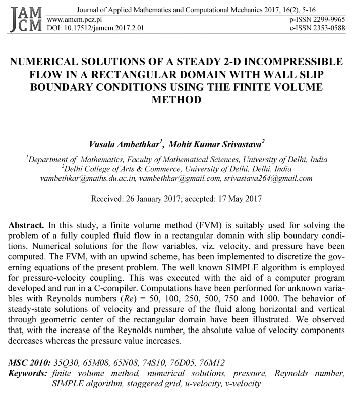
The geometry of the problem in the paper, along with the boundary conditions, is drawn in Figure 1. ABCD is a rectangular domain about the point (1, 0.5) in which a steady 2-D incompressible viscous flow is considered. Flow is set up in a rectangular domain with three stationary walls and a top lid that moves to the right with constant speed (u = 2).
At all four corner point velocities (u, v) vanish. It may be noted here regarding specifying the boundary conditions for pressure, the convention followed is that either the pressure at the boundary is given or the velocity component normal to the boundary is specified.
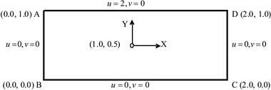
Fig. 1. The rectangular domain
2.2. Governing equations
In the present investigation, a steady 2-D incompressible fluid flow in a rectangular domain with wall slip boundary conditions has been considered. The governing equations (1)-(3) subject to the boundary conditions (4) are solved using finite volume method. The details of 4 the geometry for the configurations considered are shown in Figure 1. Taking usual Boussniesq approximations into account, the governing equations of the problem in dimensionless form
can be written as
Continuity
equation ![]() (1)
(1)
x-momentum equation ![]() (2)
(2)
y-momentum equation ![]() (3)
(3)
Boundary conditions
on boundary AB: ![]() on boundary BC:
on boundary BC:![]() (4)
(4)
on boundary CD: ![]() on boundary DA:
on boundary DA:![]()
3. Numerical method
A finite difference method (FMD) discretization is based upon the differentiable form of the PDE to be solved. The depended variables are stored at the nodes only. The FDM is easiest to understand when the geometry is regularly shaped. A finite element method (FEM) discretization is based upon a piecewise representation of the solution in terms of specified basis functions. The dependent variables are stored at finite elements nodes. The method is a mathematical approach that is difficult to put any physical significance on the terms in the algebraic equations. A Finite Volume Method (FVM) discretization is based upon an integral form of the PDE to be solved. The dependent variables are stored at the centre of the volume. The basic advantage of FVM is it does not require the use of structured grids. It is always better to use governing equation in conservative form with finite volume approach to solve any problem which ensures conservation of all the properties in each cells.
The numerical method that has been adopted
for the problem under study is the finite volume method (FVM) based on a
uniform staggered grid system. In a staggered grid [21] as shown in Figure 2,
the scalar variables, including pressure, are stored at the nodes marked ![]() . The velocities are defined at the
(scalar) cell faces in between the nodes and are indicated by arrows.
Horizontal
. The velocities are defined at the
(scalar) cell faces in between the nodes and are indicated by arrows.
Horizontal ![]() arrows indicate the locations for u-velocities
and the vertical
arrows indicate the locations for u-velocities
and the vertical ![]() ones denote those for
v-velocity. In addition to the E, W, N, S
notation, the u-velocities are stored at scalar cell faces e and
w and the v-velocities face n and s. We observe that
the finite volumes for u and v are different from the scalar
finite volumes and from each
other. The scalar finite volumes are sometimes referred to as the pressure
finite volumes because, the discrtized continuity equation is turned into a
pressure correction equation, which is evaluated on scalar finite volumes.
ones denote those for
v-velocity. In addition to the E, W, N, S
notation, the u-velocities are stored at scalar cell faces e and
w and the v-velocities face n and s. We observe that
the finite volumes for u and v are different from the scalar
finite volumes and from each
other. The scalar finite volumes are sometimes referred to as the pressure
finite volumes because, the discrtized continuity equation is turned into a
pressure correction equation, which is evaluated on scalar finite volumes.
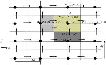 |
Fig. 2. Staggered grid
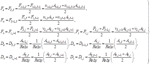
Expressed in the new co-ordinate system, the discretized u-momentum equation for the velocity at the location (i , J) is given by
| (5) |
where Ai,J is the (east or west) cell face area of the u-finite volume. In the numbering system the W, E, S and N neighbors involved in the summation ∑anbunb are (i-1, J), (i+1, J), (i, J-1) and (i, J+1). Their locations and the prevailing velocities are shown in Figure 3. The coefficients for the upwind differencing scheme are as follows:
 | (6) |
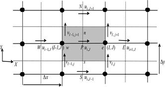 |
Fig. 3. A u-finite volume and its neighboring velocity components
The coefficients contain combinations of the convective mass flux F and the diffusive conductance D at u-finite volume cell faces. Applying the new notation system we give the values of F and D for each of the faces e, w, n and s of the u-finite volume.
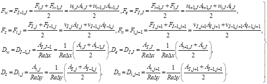 (7)
(7)
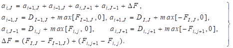
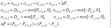
By analogy the v-momentum equation becomes
where Ai,J is the (east or west) cell face area of the v-finite volume. In the numbering system the W, E, S and N neighbors involved in the summation ∑anbvnb are (I+1, j), (I-1, J), (I, j-1) and (I, j+1). Their locations and the prevailing velocities are shown in Figure 4. The coefficients for the upwind differencing scheme are as follows:
 (9) (9) |
Fig. 4. A v-finite volume and its neighboring velocity components
The coefficients contain combinations of the convective mass flux F and the diffusive conductance D at v-finite volume cell faces. Applying the new notation system, we give the values of F and D for each of the faces e, w, n and s of the v-finite volume.
 (10)
(10)
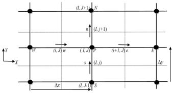 |
Fig. 5. Scalar finite volume (continuity equation)
The pressure correction equation is given by
| (11) |
where:
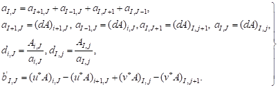 (12) (12) |
Equation (11) represents the discretized continuity
equation as an equation for pressure correction![]() . The
source term b' in the equation is the continuity imbalance arising from
the incorrect velocity field.
. The
source term b' in the equation is the continuity imbalance arising from
the incorrect velocity field.
4. Numerical computations
The acronym SIMPLE stands for Semi-Implicit Method for Pressure-Linked Equations. The algorithm is originally put forward by Patankar and Spalding [22] and essentially a guess-and-correct procedure for the calculation of pressure on a staggered grid arrangement introduced above. The algorithm gives a method of calculating pressure and velocities. The method is iterative, and when other scalars are coupled to the momentum equations the calculation needs to be done sequentially. The discretized momentum equation and pressure correction equation are solved implicitly, where the velocity correction is solved explicitly. This is the reason why it is called Semi-Implicit Method. The algorithm involves an iterative process in which the pressure correction equation is susceptible to divergence unless some under-relaxation is used. We have used a suitable under-relaxation factor to fluid out the converged values of pressure and velocities.
5. Results and discussion
In order to get clear insight into the problem, the numerical computations of u-velocity, v-velocity, the pressure for the Reynolds number by the method described under Section 3 has been done based on an algorithm given under Section 4.
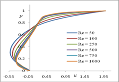
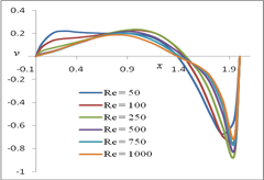
Fig. 6. u-velocity along the vertical line Fig. 7. v-velocity along the horizontal line through the geometric center of the domain through the geometric center of the domain
Figure 6 illustrates the behavior of u-velocity along the vertical line, through the geometric centre of the rectangular domain. We observed that, for a given Re, u-velocity first decreases from the bottom boundary (u = 0) and reaches its starting value (u = 0) at around the midpoint of the rectangular domain. It then increases from the midpoint to the upper boundary (u = 2). We also observed that the absolute value of u-velocity decreases with an increase in the Reynolds number. Figure 7 illustrates the behavior of v-velocity along the horizontal line, through the geometric centre of the rectangular domain. It is evident that, for a given Re, v-velocity first increases from the left boundary (v = 0) to the midpoint of the rectangular domain. Then, it decreases from the midpoint to the right boundary (v = 0). Further, the absolute value of v-velocity decreases with an increase in the Reynolds number. The origins for these graphs for various values of Reynolds numbers (Re) have been displaced for clarity of the profiles. The thinning of the wall boundary layers with an increase in Re is evident from these profiles. The near-linearity of these velocity profiles in the central core of the rectangular domain can also be observed.
Figure 8 illustrates the variation of pressure, at different grid points {(x, y) = = (0.0556, 0.5), (0.5, 0.5), (1.0556, 0.5), (1.5, 0.5), (1.9444, 0.5)}, for different Re. Figure 9 illustrates the variation of pressure, at different grid points {(x, y) = (1.0, 0.0278), (1.0, 0.2500), (1.0, 0.5278), (1.0, 0.7500), (1.0, 0.9722)}, for different Re. We observe that, the pressure increases with the increase of Re, tabulated at given grid points.
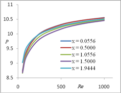
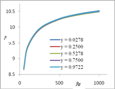
Fig. 8. Pressure variation for different Re at (y = 0.5) Fig. 9. Pressure variation for different Re at (x = 1.0)
5. Conclusions
The problem of a steady 2-D incompressible viscous flow in a rectangular domain with wall slip boundary conditions has been investigated. A finite volume method, with upwind scheme, has been employed as numerical scheme to solve the governing equations of this problem. The well known SIMPLE algorithm is employed for velocity and pressure coupling. The numerical computations for these flow variables have been obtained with the help of a code in C-programming language. Using numerical simulations, we have illustrated the variation of u-velocity along the vertical line, and v-velocity along the horizontal line through the geometric centre of the rectangular domain, at different Reynolds numbers (Re = 50, 100, 250, 500, 750, 1000). We observed that, the absolute value of velocity decreases with an increase in Reynolds number (Re). We have listed out the numerical solutions for pressure, at different Re, along the horizontal and vertical lines through geometric center of the domain respectively. We observed that, pressure increases with the increase of Reynolds number, tabulated at given grid points.
Nomenclature
x, y co-ordinates
![]() grid spacing along x
and y-axes
grid spacing along x
and y-axes
u,v horizontal and vertical component of the velocity
![]() initial guess for horizontal and vertical
component of the velocity
initial guess for horizontal and vertical
component of the velocity
P dimensionless pressure
![]() initial guess for dimensionless pressure
initial guess for dimensionless pressure
![]() pressure correction
pressure correction
![]() convective flux per unit mass at west, east, south and
north face respectively
convective flux per unit mass at west, east, south and
north face respectively
![]() diffusivity conductance at west, east, south and north face
respectively
diffusivity conductance at west, east, south and north face
respectively
Subscript
i, j index used in tensor notation
nb neighboring coordinate
e finite volume face P and E
w finite volume face P and W
n finite volume face P and N
s finite volume face P and S
Acknowledgement
The authors acknowledge the support from the Council of Scientific and Industrial Research (HRDG, Government of India) for providing research grant under SRF wide letter no. 09/045(0906)/2009-EMR-I to carry out this work.
References
[1] Patankar S.V., Numerical Heat Transfer and Fluid Flow, Hemisphere, New York 1980.
[2] Anderson D.A., Pletcher R.H., Tannehill J.C., Computational Fluid Mechanics and Heat Transfer, Second ed., Taylor and Francis, Washington D.C. 1997.
[3] Bozeman J.D., Dalton C., Numerical study of viscous flow in a cavity, Journal of Computational Physics 1973, 12, 348-363.
[4] Ghia U., Ghia K.N., Shin C.T., High-Re solutions for incompressible flow using the Navier- -Stokes equations and a multigrid method, Journal of Computational Physics 1982, 48, 387-411.
[5] Bruneau C.H., Jouron C., An efficient scheme for solving steady incompressible Navier-Stokes equations, Journal of Computational Physics 1990, 89, 389-413.
[6] Mansour M.L., Hamed A., Implicit solution of the incompressible Navier-Stokes equations on non-staggered grid, Journal of Computational Physics 1990, 86, 147-167.
[7] Spotz W.F., Accuracy and performance of numerical wall boundary conditions for steady 2-D incompressible stream function vorticity, International Journal for Numerical Methods in Fluids 1998, 28, 737-757.
[8] Boivin S., Cayre F., Herard J.M., A finite volume method to solve the Navier-Stokes equations for incompressible flows on structured meshes, International Journal of Thermal Sciences 2000, 39, 806-825.
[9] Kalita J.C., Dalal D.C., Dass A.K., Fully compact higher-order computation of steady-state natural convection in a square cavity, Physical Review E 2001, 64, 066703.
[10] Liakos A., Discretization of the Navier-Stokes equations with slip boundary condition, Numerical Methods for Partial Differential Equations 2001, 17, 26-42.
[11] Piller M., Stalio E., Finite-volume compact schemes on staggered grids, Journal of Computational Physics 2004, 197, 299-340.
[12] Oztop H.F., Dagtekin I., Mixed convection in two-sided lid-driven differentially heated square cavity, International Journal of Heat and Mass Transfer 2004, 47, 1761-1769.
[13] Erturk E., Corke T.C., Gokcol C., Numerical solutions of 2-D steady incompressible driven cavity flow at high Reynolds numbers, International Journal for Numerical Methods in Fluids 2005, 48, 747-774.
[14] Young D.L., Jane S.J., Fan C.M., Murugesan K., Tsai C.C., The method of fundamental solutions for 2D and 3D Stokes problems, Journal of Computational Physics 2006, 211, 1-8.
[15] Droniou J., Eymard R., A mixed finite volume scheme for anisotropic diffusion problems on any grid, Numer. Math. 2006, 105, 35-71.
[16] Salem S.A., On the numerical solution of the incompressible Navier-Stokes equations in primitive variables using grid generation techniques, Mathematical and Computational Applications 2006, 11, 127-136.
[17] Mencinger J., Zun I., On the finite volume discretization of discontinuous body force field on collocated grid: Application to VOF method, Journal of Computational Physics 2007, 221, 524- -538.
[18] Bharti R.P., Chhabra R.P., Eswaran V., A numerical study of steady forced convection heat transfer from an unconfined circular cylinder, Heat Mass Transfer 2007, 43, 639-648.
[19] Hokpunna A., Manhart M., Compact fourth-order finite volume method for numerical solutions of Navier-Stokes equations on staggered grids, Journal of Computational Physics 2010, 229, 7545-7470.
[20] Sathiyamoorthy M., Chamkha A.J., Effect of magnetic field on natural convection flow in a liquid gallium filled square cavity for linearly heated side wall(s), International Journal of Thermal Sciences 2010, 49, 1856-1865.
[21] Versteeg H.K., Malalsekra W., An Introduction to Computational Fluid Dynamics: The Finite Volume Method, Second ed., Pearson, India 2007.
[22] Patankar S.V., Spalding D.B., A calculation procedure for heat, mass and momentum transfer in three-dimensional parabolic flows, Int. J. Heat Mass. Transfer 1972, 15, 1787.