Redefinition of triad's inconsistency and its impact on the consistency measurement of pairwise comparison matrix
Paweł Tadeusz Kazibudzki
Journal of Applied Mathematics and Computational Mechanics |
 Download Full Text |
REDEFINITION OF TRIAD’S INCONSISTENCY AND ITS IMPACT ON THE CONSISTENCY MEASUREMENT OF PAIRWISE COMPARISON MATRIX
Paweł Tadeusz Kazibudzki
Institute of
Management and Marketing, Jan Dlugosz University in Czestochowa
Częstochowa, Poland
p.kazibudzki@ajd.czest.pl
Abstract. There is a theory which meets a prescription of the efficient and effective multicriteria decision making support system called the Analytic Hierarchy Process (AHP). It seems to be the most widely used approach in the world today, as well as the most validated methodology for decision making. The consistency measurement of human judgments appears to be the crucial problem in this concept. This research paper redefines the idea of the triad’s consistency within the pairwise comparison matrix (PCM) and proposes a few seminal indices for PCM consistency measurement. The quality of new propositions is then studied with application of computer simulations coded and run in Wolfram Mathematica 9.0.
Keywords: AHP, pairwise comparisons, consistency, judgments, Monte Carlo simulations
1. Introduction
There is a methodology which meets prescriptions for efficient and effective multiple criteria decision making (MCDM) process. It is called the Analytic Hierarchy Process (AHP) and was developed at the Wharton School of Business by Thomas Saaty [1]. The AHP seems to be the most widely used MCDM approach in the world today, as well the most validated methodology. There are thousands of actual applications in which the AHP results were accepted and used by the competent decision makers (DM). Thorough reviews of the contemporary applications and developments in the AHP can be found for example in [2-5].
The AHP allows DM to set priorities and make choices on the basis of their objectives, knowledge and experiences in a way that is consistent with their intuitive thought process. The process permits accurate priorities to be derived from verbal judgments even though the words themselves may not be very precise. That is why special attention is given to issues associated with consistency of DM judgments. However, inconsistency results not only due to DM inaccuracy in their judgments but also due to existing scales, which must be utilized in order to enable DM to somehow express their fuzzy preferences.
2. Mathematics behind the Analytic Hierarchy Process
The conventional procedure of priorities ranking in AHP is grounded on the well-defined mathematical structure of consistent matrices and their associated right-eigenvector’s ability to generate true or approximate weights [1, 5]. It was proved that, if A = (wij), wij > 0, where i, j = 1,…, n, then A has a simple positive eigenvalue lmax called the principal eigenvalue of A and lmax > |lk | for the remaining eigenvalues of A. Furthermore, the principal eigenvector w = [w1,…, wn]T that is a solution of Aw = lmaxw has wi > 0, i = 1,…, n. If we know the relative weights of a set of activities we can express them in a pairwise comparison matrix (PCM) denoted as A(w). Now, knowing A(w) but not w (vector of priorities) we can use Perron’s theorem and solve this problem for w.
Definition 1. If the elements of a matrix A(w) satisfy the condition wij = 1/wji for all i, j = 1,…, n, then the matrix A(w) is called reciprocal.
Definition 2. If the elements of a matrix A(w) satisfy the condition wikwkj = wij for all i, j, k = 1,…, n, and the matrix is reciprocal, then it is called consistent or cardinally transitive.
Thus, the conventional concept of AHP can be presented as: A(w) w = n w. When AHP is utilized in real life situations we do not have A(w) which would reflect priority weights given by the vector of priorities. Thus, we do not have A(w) but only its estimate A(x). In such a case the consistency property does not hold and the relation between elements of A(x) and A(w) can be expressed as follows:
| (1) |
where eij is a perturbation factor nearby unity. In the statistical approach eij reflects a realization of a random variable with a given probability distribution.
Thus, in order to analyze the consistency of decision makers’ judgments, Saaty proposes measuring the inconsistency of data contained in the PCM by a consistency index CI(n) computed according to the following formula:
| (2) |
However, very recent developments in the field exposed the necessity for further analysis in this area because Saaty’s index can be a very misleading one.
3. Description of the problem and its solution
It should be realized here that we have three significantly different notions:
– the PCM consistency perceived from a perspective of the Definition 2, and expressed by the specific inconsistency index value,
– the consistency of decision makers, i.e. their trustworthiness, reflected by the number and size of their judgments discrepancies, and
– the PCM applicability for estimation of decision makers’ priorities in the way that leads to minimization of their estimation errors.
As it seems, the third issue is probably the most important problem in the contemporary arena of the MCDM theory concerning AHP, and the only way to examine that phenomena is through computer simulations.
Saaty insists that the consistency index CI(n) is necessary and sufficient to uniquely capture the consistency inherent in pairwise comparison judgments. However, there are many other procedures devised in order to cope with this problem. They are connected with various other priorities estimation procedures that exist, and can be found in the literature, e.g. Logarithmic Least Squares Method (LLSM) [6] given by the formula:
| (3) |
and connected with it the consistency index (CILLSM) given by the formula:
| (4) |
Many of these procedures are optimization based and seek a vector w as a solution of the minimization problem given by the formula:
| min D | (A(x), A(w)) (5) |
subject to some assigned constraints such as for example positive coefficients and normalization condition. Because the distance function D measures an interval between matrices A(x) and A(w), different ways of its definition lead to different prioritization concepts, prioritization results and consistency measures [7]. Further- more, since the publication of [7] a few other procedures were introduced to the literature along with their consistency measures concepts, i.e.: the procedure based on the goal programming approach [8], and a few based on constrained optimization models [9, 10].
However, there is a consistency index that is not connected with any prioritization procedure, and this index was devised by Koczkodaj [11], which attracts our special attention. In order to understand its essence we must explain the notion of a triad. It is a fact that for any three distinguished decision alternatives there are three meaningful priority ratios (denoted hereafter as: a, b, c), which have their different locations in a particular PCM (denoted as: A(x) = [xij]nxn). Now, if a = aik, c = akj, b = aij for some different i £ n, j £ n, and k £ n, the tuple (a, b, c) is called a triad. Certainly, in every consistent PCM, for all triads the following equality holds: ac = b. Thus, equations 1 – b/ac = 0 and 1 – ac/b = 0 must be true in such circumstances. Applying this principle, Koczkodaj introduced his index denoted as: TI (a, b, c) intended for measurement of triad’s consistency, given by the formula:
| (6) |
and following this idea he proposed the following index KI(TI) designated to measure consistency of any reciprocal PCM:
| (7) |
where the maximum value of TI (a, b, c) is taken from the set of all possible triads in the upper triangle of a given PCM.
The fact that Koczkodaj’s index is not connected with any prioritization procedure makes it especially attractive. Furthermore, it is possible to redefine that index and make it less complicated from the viewpoint of mathematical applications.
That is why we propose two new indices for characterization of the triad’s consistency which allow us to simplify computations and consider only one component within the index instead of searching for a minimum of two as in the case of TI (a, b, c). Following the idea, that ln(ac/b) = –ln(b/ac), instead of TI (a, b, c), we suggest two seminal formulae intended for measurement of triad’s consistency, denoted as LTI (a, b, c) and LTI* (a, b, c), defined by the two following equations:
| (8) |
| (9) |
We can now suggest two new indices for the purpose of consistency measurement of any PCM, given by the following formulae (simplifying, LTI therein denotes alternatively LTI (a, b, c) or LTI* (a, b, c)):
| (10) |
| (11) |
where the above measures (10) and (11) can be computed on the basis of all different triads (a, b, c) not necessarily in the upper triangle of the given PCM which in this case can be reciprocal or nonreciprocal.
In order to verify if the above presented indices qualify for the assessment of the PCM applicability for estimation of the decision makers’ priorities in the way that leads to minimization of their estimation errors, we would like to verify their performance with the help of Monte Carlo simulations. It is the fact that Monte Carlo simulations are commonly recognized as important and credible source of scientific information [12]. They are applied for examination purposes of various phenomena, e.g.: consequences of decisions made, or different processes subdued to random impact of the particular environment [13].
4. Computer simulations of the selected index performance
In order to evaluate a performance of earlier proposed indices, we designed the following simulation scenario. In agreement with assumptions described in Grzybowski [14] it is possible to design and execute the simulation algorithm comprising the following steps:
Step 1. Randomly generate a priority vector k = [k1,…, kn]T of assigned size [nx1] and related perfect PCM(k) = K(k).
Step 2. Randomly choose an element kxy for x < y of K(k) and replace it with kxyeB where eB is relatively a significant error which is randomly drawn from the interval DB with assigned probability distribution p.
Step 3. For each other element kij, i < j £ n randomly choose a value eij for the small error in accordance with the given probability distribution p and replace the element kij with the element kij eij.
Step 4. Round all values of kij eij for i < j of K(k) to the closest value from a considered scale.
Step 5. Replace all elements kij for i > j of K(k) with 1/kij.
Step 6. After all replacements are done, calculate the value of the examined index as well as the estimates of the vector k denoted as k*(EP) with application of assigned estimation procedure (EP). Then compute estimates errors AE(k*(EP), k) and RE(k*(EP), k) denoting the absolute and relative error respectively. Remember values computed in this step as one record.
Step 7. Repeat Steps 2 to 6 NM times.
Step 8. Repeat Steps 2 to 7 NR times.
Step 9. Return all records organized as one database.
The probability distribution p attributed in Step 3 to the perturbation factor eij is applied in equal proportions as: gamma, log-normal, truncated normal, and uniform distribution. These are four of the distribution types, which are most frequently considered in literature for various implementation purposes.
Our simulation scenario assumes that the perturbation factor eij will be drawn from the interval e Î[0.5;1.5]. Noticeably, in the simulation scenario, parameters of implemented probability distributions are set in such a way that the expected value of eij equals unity. The latter assumption seems very reasonable because human judgments are not accurate, nevertheless undeniably they circle nearby perfect ones. The “big error”, applied in Step 2, has the uniform distribution on the interval eB Î[2;4].
Due to necessity of diminishing the volume of this paper we will present only results for MLTI(LTI) and only for n = 4. For the same reason we selected only LLSM as the procedure applied for estimation purposes, thus in our simulations EP = LLSM. Our simulation scenario also assumes application of the rounding procedure which in this research operates according to Saaty’s scale. It comprises the integers from one (equivalent to the verbal judgment: “equally preferred”) to nine (equivalent to the verbal judgment: “extremely preferred”) and their reciprocals.
Finally, our scenario takes into account the obligatory assumption in conventional AHP applications, i.e.: the PCM reciprocity condition. In such cases only judgments from the upper triangle of a given PCM are taken into account and those from the lower triangle are replaced by the inverses of the former ones. The outcome of the simulation scenario present Table 1 and Figures 1, 2. Distinguished plots within Figures 1 and 2 present relations between average MLTI(LTI) and p-quantiles or average AE(LLSM) with Spearman rank correlation coefficients (SRCC).
Table 1
Performance of the index MLTI(LTI) in relation to AE(LLSM) distribution
|
Average MLTI |
p-quantiles of AE(LLSM) |
Average AE(LLSM) |
||
|
p = 0.1 |
p = 0.5 |
p = 0.9 |
||
|
0.426707 |
0.0104028 |
0.0325444 |
0.0693912 |
0.0370195 |
|
0.750337 |
0.0157984 |
0.0411051 |
0.0791007 |
0.0451398 |
|
0.990685 |
0.0161317 |
0.0438768 |
0.0809734 |
0.0472575 |
|
1.223530 |
0.0162664 |
0.0438350 |
0.0846752 |
0.0481755 |
|
1.449600 |
0.0159626 |
0.0475032 |
0.0887029 |
0.0511369 |
|
1.690140 |
0.0171854 |
0.0471083 |
0.0908819 |
0.0518714 |
|
1.927420 |
0.0190256 |
0.0487652 |
0.0926036 |
0.0538121 |
|
2.159650 |
0.0183335 |
0.0483145 |
0.0951448 |
0.0540101 |
|
2.395130 |
0.0193643 |
0.0487246 |
0.0999413 |
0.0555574 |
|
2.637340 |
0.0188251 |
0.0479729 |
0.1001040 |
0.0550359 |
|
2.876040 |
0.0197419 |
0.0505363 |
0.1067170 |
0.0584622 |
|
3.102830 |
0.0195147 |
0.0518240 |
0.1088690 |
0.0598924 |
|
3.333710 |
0.0224324 |
0.0584043 |
0.1148840 |
0.0648018 |
|
3.575140 |
0.0192635 |
0.0577230 |
0.1220180 |
0.0646491 |
|
4.267770 |
0.0212392 |
0.0607142 |
0.1353990 |
0.0711039 |
Note: results based on 40 000 random reciprocal PCMs
|
|
|
|
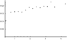
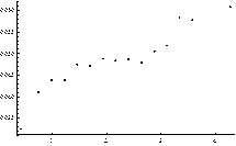
Fig. 1. Performance of the index MLTI(LTI). Plot of correlation between average values of MLTI(LTI) and: AE quantiles of order p = 0.1 (Plot A) and p = 0.5 (Plot B)
|
|
|
|
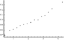
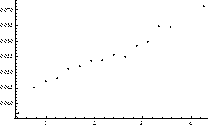
Fig. 2. Performance of the index MLTI(LTI). Plot of correlation between average values of MLTI(LTI) and: AE quantiles of order p = 0.9 (Plot A) and the average AE (Plot B)
5. Conclusions
We can see that the relation between the average value of MLTI(LTI) and analyzed statistics is more or less monotonic. This is a very positive message from the perspective of the PCM applicability evaluation for estimation of decision makers’ priorities in the way that leads to minimization of their estimation errors. Our attention especially attracts the fact that the mean value of MLTI(LTI) and the quantile of order 0.9 are perfectly monotonic (SRCC = 1). It is worth mentioning here that the same characteristics perform slightly worse when CI(LLSM) was examined.
The monotonic relationship between the values of MLTI(LTI) and the quantiles as well as mean absolute errors (AE) is especially compelling from the perspective of this research study. It is so because these quantiles can be used to accept or reject particular PCM as a good or bad source of information. Thus, both quantiles of order 0.1 and 0.9 provide some knowledge about a prospective outcome we may achieve when the process of estimation is finished.
We feel that new measurements introduced herein concerning the PCM applicability evaluation for estimation of decision makers’ priorities in the way that leads to the minimization of their estimation errors, either have potential to become a subject of further analysis and research studies. From the perspective of this research study both LTI (a, b, c) and MLTI(LTI) are quite good indicators of the trustworthiness of the PCM as a source of information about the priority vector.
Recapitulating, we proposed some new indices for the triad’s consistency measurement which, in our opinion, have better prospects than for example CI(LLSM). It should be underlined here that they are simpler than Koczkodaj’s proposition which makes them especially attractive from the perspective of further more formal, mathematical analysis.
It is crucial to also examine other consistency measures proposed in this paper which were not examined here (due to article’s volume constraint) and also find out their performance in relation to other known prioritization procedures and other values for n. Special attention must be given to the issue, if these measures grow in value simultaneously with the growth of estimation errors.
We intend to undertake research studies concerning these issues and hopefully plan to report about their results in the near future.
References
[1] Saaty T.L., A scaling method for priorities in hierarchical structures, J. Math. Psycho. 1977, June, 15, 234-281.
[2] Ishizaka A., Labib A., Review of the main developments in the analytic hierarchy process, Expert Syst. Appl. 2011, 11(38), 14336-14345.
[3] Ho W., Integrated analytic hierarchy process and its applications - A literature review, Euro. J. Oper. Res. 2008, 186, 211-228.
[4] Vaidya O.S., Kumar S., Analytic hierarchy process: An overview of applications, Euro. J. Oper. Res. 2006, 169, 1-29.
[5] Saaty T.L., Fundamentals of Decision Making and Priority Theory with the Analytic Hierarchy Process, RWS Publication, Pittsburgh, PA 2006.
[6] Crawford G., Williams C.A., A note on the analysis of subjective judgment matrices, J. Math. Psychol. 1985, 29, 387-405.
[7] Choo E.U., Wedley W.C., A common framework for deriving preference values from pairwise comparison matrices, Comp. Oper. Res. 2004, 31, 893-908.
[8] Grzybowski A.Z., Goal programming approach for deriving priority vectors - some new ideas, Scientific Research of the Institute of Mathematics and Computer Science 2010, 1(9), 17-27.
[9] Grzybowski A.Z., Note on a new optimization based approach for estimating priority weights and related consistency index, Expert Syst. Appl. 2012, 39, 11699-11708.
[10] Grzybowski A.Z., New optimization-based method for estimating priority weights, Journal of Applied Mathematics and Computational Mechanics 2013, 12(1), 33-44.
[11] Koczkodaj W.W., A new definition of consistency of pairwise comparisons, Mathematical and Computer Modeling 1993, 18(7), 79-84.
[12] Winsberg E.B., Science in the Age of Computer Simulations, The University of Chicago Press, Chicago 2010.
[13] Grzybowski A., Domański Z., A sequential algorithm for modeling random movements of chain-like structures, Scientific Research of the Institute of Mathematics and Computer Science 2011, 10(1), 5-10.
[14] Grzybowski A.Z., New results on inconsistency indices and their relationship with the quality of priority vector estimation, Expert Syst. Appl. 2016, 43, 197-212.