Galerkin method for bending analysis of beams on non-homogeneous foundation
Abubakr E.S. Musa
Journal of Applied Mathematics and Computational Mechanics |
 Download Full Text |
GALERKIN METHOD FOR BENDING ANALYSIS OF BEAMS ON NON-HOMOGENEOUS FOUNDATION
Abubakr E.S. Musa
Department of Civil and Environmental
Engineering, King Fahd University
of Petroleum and Minerals
Dhahran, Saudi Arabia
bakri083@gmail.com
Received: 23 February 2017; Accepted: 14 July 2017
Abstract. In this study, a mathematical formulation for static bending analysis of a beam on a non-homogenous foundation is presented. The proposed method offers an accurate procedure for analysis and design of a beam resting on a varying soil bed. The Winkler foundation model is used and presented using discontinuous functions to account for the sudden change in the soil stiffness coefficient. The solution of the governing differential equation is then obtained using the Galerkin method with the help of approximation functions that satisfy the boundary conditions. A systematic approach for setting the approximation functions for different support and soil conditions is suggested. The accuracy of the proposed method is verified through two numerical examples, and they showed an excellent agreement with the finite element method (FEM) and available literature results.
MSC: 65L60, 74S05
Keywords: Galerkin method, non-homogenous foundation, analysis of beams, beam on elastic foundation
1. Introduction
Bending analysis of beams or plates in elastic foundation is used extensively in engineering practice as far as soil-structure interaction is concerned. The backbone of this analysis is modelling the contact pressure between the structural member and the soil bed. Upon the assumed behavior of deformation of the soil under loading, different models are presented to introduce the effect of the soil medium. Some of these models are the one parameter foundation or the Winkler model [1] and two parameters model such as Hetenyi [2] and Pasternak [3] where other springs interacting with the vertical ones are considered.
Analysis of the beam on the elastic foundation model started early on by different researchers [4-8]. Other types of foundation models have also been covered extensively such as a beam resting on a visco-elastic foundation, which has been studied by Sonoda et al. [9] and a beam on nonlinear foundation has also been studied [10]. On the other hand, and in addition to the classical beam theory, some researchers went further to study the analysis of Timoshenko’s beam on an elastic foundation considering the effect of shear deformation as it was studied in [11-13]. Moreover, the computer coding, as a power of solving many engineering problems, has also been utilized in the analysis of the beam on an elastic foundation as it has been presented by Teodorue [14], who developed a new computer code based on FEM for a beam on an elastic foundation using Matlab software, making it easy to perform different kinds of problems with slight changes in the input data.
In many engineering problems, it is very common to have discontinuity in the loading and the geometrical properties of the beam. Some researchers followed this trend as the study of Yavari et al. [15] for the problem of a beam with loading and geometrical discontinuity. The expression of loading conditions in terms of discontinuous functions was also covered [16] making the treatment of different types of loads easy to handle, and the solution of the governing differential equation was observed using Wolfram Mathematica.
In many construction sites, and without the excessive soil stabilization process, the soil bed is, most likely, found to have different mechanical properties such as bearing capacity and soil subgrade reaction. A comprehensive treatment is, therefore, required to make the soil bed more homogenous. Alternatively, it is very necessary to consider the non-homogeneity conditions of the soil bed in the design stage to account for the associated stresses. This phenomenon of a beam on non-homogenous foundation was studied and presented [17, 18]. In addition, the design of spread foundation resting on a soil with geological anomaly has also been reported in 2014 [19]. In this latest study, the one dimensional model and the three-dimensional model were studied, but in both cases the finite element was used for the analysis process.
In this study, an Euler beam resting on a one-parameter foundation of varying subgrade reaction is presented. The use of discontinuous functions makes it easy to account for a sudden change of subgrade reaction and has a large variety of soil changes within the length of the beam but introduces a new form of difficulty to obtain an analytical solution. The governing differential equation is, therefore, solved using the Galerkin method with a set of approximation functions that satisfy the boundary conditions of the beam. These functions are to be selected using a suggested systematic approach that works for nearly any type of boundary conditions. The results of the proposed method are found to be in an excellent agreement with FEM and the results developed in the literature.
2. Mathematical formulation
The governing differential equation of a beam on an elastic foundation is presented in the first part of this section. The Galerkin method and the suggested systematic approach for generation of the approximation functions are presented in the second and third parts of this section, respectively.
2.1. The governing differential equation
Consider a beam resting on the non-homogenous
foundation as shown in Figure 1. The governing differential equation of a beam
resting on a foundation with soil stiffness coefficient ![]() and subjected to load
and subjected to load ![]() is given by
is given by
| (1) |
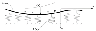
Fig. 1. Typical beam on non-homogenous foundation model
Four boundary conditions are required to
solve Eq. (1), and they can be determined according to the physics of the
problem. Other beam variables; bending moment ![]() , shear force
, shear force ![]() , and slope
, and slope ![]() can be found by the following expressions:
can be found by the following expressions:
|
|
|
|
2.2. Solution formulation
Let us select the origin of the ![]() -coordinate to be at the center of the beam, and let
-coordinate to be at the center of the beam, and let ![]() approximate the
solution of the of the governing differential equation over the beam domain and
approximate the
solution of the of the governing differential equation over the beam domain and
![]() are constants.
are constants.
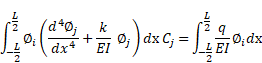
Using the assumed approximated solution ![]() in Eq. (1) results in
in Eq. (1) results in
|
|
|
where ![]() is the residual. The unknown parameters can be found by setting the
weighing average over the computational domain to zero. Leading to
is the residual. The unknown parameters can be found by setting the
weighing average over the computational domain to zero. Leading to
|
|
where ![]() is the weighing
function and its selection depends on the selected method of the solution.
Using the Galerkin method,
is the weighing
function and its selection depends on the selected method of the solution.
Using the Galerkin method, ![]() where
where ![]() satisfy all the
boundary conditions. Eq. (3) can therefore be written as
satisfy all the
boundary conditions. Eq. (3) can therefore be written as
|
(4) |
Use of Eqs. (2) and (4) yields
|
(5) |
Substitution of ![]() into Eq. (5) and
simplifying yields
into Eq. (5) and
simplifying yields
|
(6) |
which can be written in the following matrix form
|
|
(7) |
where
 |
and
 |
2.3. Selection of the approximation functions
The selection
procedure of the approximation functions satisfy all the four boundary
conditions requiring a clear understanding of the physics of the beam problem
under consideration. In this paper, some hints and examples of how to
select these functions ![]() are given.
are given.
The elastic
foundation considered here might take a different form of variation, including
a sudden change in the soil subgrade reaction such as presence of geological
anomaly in the construction site. The beam can also be partially supported by
the soil such as presence of void or a cavity zone under the beam. Modeling of
these types of subgrade reactions can be expressed with the help of
discontinuous functions such as Heaviside functions. Other forms of variations
may include any form of continuous functions. The function that represents the
subgrade reaction should be set prior to selection of the approximation
functions ![]() .
.
Since the
approximation functions must satisfy the boundary conditions, let us start by
the three beams shown in Figure 2. These three beams have the same zero
deflection at their boundaries but differ in the other boundary conditions.
This makes it possible to set a systematic approach to find the function ![]() for these three cases.
Let us introduce a starting function
for these three cases.
Let us introduce a starting function ![]() to take the form
to take the form
|
|
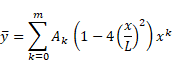
which
satisfies the zero deflection boundary conditions for the three shown cases.
The remaining two boundary conditions for each case can be satisfied by forcing
the function ![]() to satisfy the
remaining two boundary conditions. This results in two equations and can be
utilized to express two of the constants in terms of the others leading to a
function
to satisfy the
remaining two boundary conditions. This results in two equations and can be
utilized to express two of the constants in terms of the others leading to a
function ![]() satisfying all the
boundary conditions and number of
satisfying all the
boundary conditions and number of ![]() unknown constants
unknown constants ![]() .
.
Organization of
the resultant function ![]() and separating it into
constants multiplied by functions of
and separating it into
constants multiplied by functions of ![]() leads to
leads to ![]() constant multiplied by the same number of functions. Then renaming
these functions to be
constant multiplied by the same number of functions. Then renaming
these functions to be ![]() and the constants to
be
and the constants to
be ![]() for
for ![]() where
where ![]() It is noteworthy that
It is noteworthy that ![]() satisfying all the
boundary conditions and then Eq. (7) can be applied to solve for the unknown
satisfying all the
boundary conditions and then Eq. (7) can be applied to solve for the unknown ![]() .
.
|
|
|
|
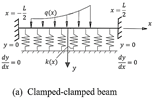
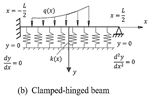
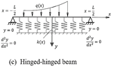
Fig. 2. Three beams on non-homogenous foundations and different boundary conditions
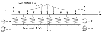
One more example is the free-free beam shown
in Figure 3. In this problem, due to symmetrical loading and the foundation
condition, it is known, as a priori, that the solution will be symmetric, and
the beam will have some deflection at the ends. The starting function ![]() can, therefore, take
the form
can, therefore, take
the form
|
|
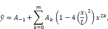
where the constant ![]() to account for the
constant deflection at the ends of the beam. The total number of constants in
the above equation is
to account for the
constant deflection at the ends of the beam. The total number of constants in
the above equation is ![]() . Due to the symmetry
property, in this problem, forcing the function
. Due to the symmetry
property, in this problem, forcing the function ![]() to satisfy four
boundary conditions results, in fact, in only two equations and, therefore,
expressing only two constants in terms of others. Again, organizing the
remaining constants and their accompanying functions yields in
to satisfy four
boundary conditions results, in fact, in only two equations and, therefore,
expressing only two constants in terms of others. Again, organizing the
remaining constants and their accompanying functions yields in ![]() number of constants and a similar number of functions. Then,
renaming these functions to be
number of constants and a similar number of functions. Then,
renaming these functions to be ![]() and the constants to
be
and the constants to
be
![]() for
for ![]() and
and ![]() .
.
|
|
|
Fig. 3. Free-free beam on non-homogenous symmetrical foundation and subjected to symmetric loading |
A similar approach can be used to develop
approximation functions ![]() for different beam
problems. A convergence process is required to decide on the proper number of
terms
for different beam
problems. A convergence process is required to decide on the proper number of
terms ![]() , of the starting function
, of the starting function
![]() at which the
polynomial should be truncated. The convergence procedure has been presented as
shown in the next section.
at which the
polynomial should be truncated. The convergence procedure has been presented as
shown in the next section.
The aforementioned procedure of finding the
approximation functions can easily be programed in a small computer code. Then,
the obtained approximation functions can be used in Eq. (7) to solve for the
unknown variables ![]() The complete solution
The complete solution ![]() can then be found by
summing over the dummy index
can then be found by
summing over the dummy index ![]() . Other beam variables
such as shear force and bending moment can be found using the obtained
deflection expression as explained earlier.
. Other beam variables
such as shear force and bending moment can be found using the obtained
deflection expression as explained earlier.
3. Numerical examples
Application of the developed method has been explained through two numerical examples. The accuracy of the obtained results is verified with those obtained by FEM and the available results in the literature.
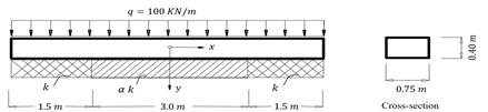
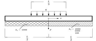
3.1. Example 1: A foundation of a load bearing wall of finite length constructed on soil of non-homogenous subgrade reaction
A
load bearing wall of total constant uniformly distributed load of
![]() resting on non-homogenous foundation having a subgrade reaction
resting on non-homogenous foundation having a subgrade reaction ![]() at
the outer quarters and
at
the outer quarters and ![]() at the middle part as shown in Figure 4. The numerical value of the
subgrade reaction for the outer quarters per unit length of the foundation is
at the middle part as shown in Figure 4. The numerical value of the
subgrade reaction for the outer quarters per unit length of the foundation is ![]() , and the values of
, and the values of ![]() that control the subgrade
reaction of the middle part are taken to be
that control the subgrade
reaction of the middle part are taken to be ![]() and
and
![]() . The elastic modulus
of the material
. The elastic modulus
of the material ![]() .
.
|
|
|
Fig. 4. A foundation of load bearing wall on non-homogenous subgrade reaction |
The subgrade reaction modulus, in this problem, can be expressed using the discontinuous function to take the form
where the discontinuous function ![]() is
defined by
is
defined by
A proper way of modeling this structural member is
a free-free beam on non-homogenous foundation model. As explained in Subsection
2.3, Eq. (9) has been used in this problem as a starting point to find the
function ![]() . A convergence study to decide on the proper number of terms
. A convergence study to decide on the proper number of terms ![]() ,
after which the expression given by Eq. (9) is truncated, has been done for all
values of
,
after which the expression given by Eq. (9) is truncated, has been done for all
values of ![]() . However, for
simplicity, the convergence results have been presented only for the highest
and lowest selected values of
. However, for
simplicity, the convergence results have been presented only for the highest
and lowest selected values of ![]() . From the convergence study, only six terms are found to be enough
to truncate the number of terms
. From the convergence study, only six terms are found to be enough
to truncate the number of terms ![]() .
.
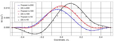
For the purpose of evaluating the accuracy of the
proposed method, the results are compared with the FEM prepared model. To
reduce the information in the figures, the FEM results are shown for only two
values of ![]() (
(![]() and
and ![]() ).
Figures 5 and 6 show an excellent agreement between the proposed Galerkin
method and FEM obtained results for the shown two models. The results of the
shear force (Fig. 7) show a moderately good agreement with FEM but it is not as
excellent as the deflection and bending moment. This less accuracy is due to
higher derivatives associated with the shear force, which makes the shear force
results have the worst agreement with FEM as compared to deflection and bending
moment, and also slower convergence rate as shown in Table 1.
).
Figures 5 and 6 show an excellent agreement between the proposed Galerkin
method and FEM obtained results for the shown two models. The results of the
shear force (Fig. 7) show a moderately good agreement with FEM but it is not as
excellent as the deflection and bending moment. This less accuracy is due to
higher derivatives associated with the shear force, which makes the shear force
results have the worst agreement with FEM as compared to deflection and bending
moment, and also slower convergence rate as shown in Table 1.
|
|
|
Fig. 5. The deflection of the free-free beam under symmetrically non-homogenous foundation model |
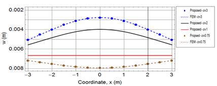
Figure 5 confirms that a free-free beam subjected
to constant load and resting on a soil of homogenous subgrade reaction (![]() portrays
a constant deflection equal to
portrays
a constant deflection equal to ![]() leading, therefore, to zero bending moment and shear force as shown
in Figures 6 and 7. The bending and shear stresses, however, appear with the
variation of subgrade reaction along the length of the beam. As a priori
construction, the deflection reduces with reduction of subgrade reaction. The
results for higher values of
leading, therefore, to zero bending moment and shear force as shown
in Figures 6 and 7. The bending and shear stresses, however, appear with the
variation of subgrade reaction along the length of the beam. As a priori
construction, the deflection reduces with reduction of subgrade reaction. The
results for higher values of ![]() show a low deflection at center of the beam and more deflection as
going to the ends of the beam leading to tensile bending stress at the top of
the beam. The negative bending moment resulting from higher subgrade reaction
at the middle (
show a low deflection at center of the beam and more deflection as
going to the ends of the beam leading to tensile bending stress at the top of
the beam. The negative bending moment resulting from higher subgrade reaction
at the middle (![]() as shown in Figure 6
requires reinforcing the top of the beam to account for the resulting tensile
stress. Furthermore, the direction of bending moment reverses its direction for
as shown in Figure 6
requires reinforcing the top of the beam to account for the resulting tensile
stress. Furthermore, the direction of bending moment reverses its direction for
![]() leading to a bottom
reinforcement requirement with an amount proportional to the reduction of
leading to a bottom
reinforcement requirement with an amount proportional to the reduction of ![]() .
.
|
|
|
|
Fig. 6. The bending moment of the free-free beam under symmetrically non-homogenous foundation model |
|
|
|
|
|
Fig. 7. The shear force of the free-free beam under symmetrically non-homogenous foundation model |
|
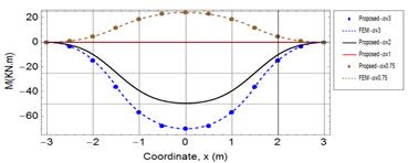
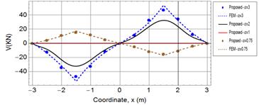
Table 1
Convergence study of Example 1
|
|
|
|
||||
|
|
|
|
|
|
|
|
|
1 |
3.33 |
0 |
0.00 |
7.62 |
0.00 |
0.00 |
|
2 |
2.78 |
‒69.47 |
34.73 |
7.94 |
23.20 |
‒11.60 |
|
3 |
2.77 |
‒73.10 |
39.12 |
7.94 |
24.81 |
‒13.51 |
|
4 |
2.77 |
‒71.40 |
42.50 |
7.94 |
24.42 |
‒14.25 |
|
5 |
2.77 |
‒70.28 |
46.73 |
7.94 |
24.11 |
‒15.42 |
|
6 |
2.77 |
‒70.15 |
46.82 |
7.94 |
24.07 |
‒15.45 |
3.2. Example 2: A free-free beam of a partially distributed load resting on non-homogenous foundation
A free-free beam subjected to a partially
distributed load at its middle third and resting on a non-homogenous foundation
as shown in Figure 8. The main purpose of presenting this example is to verify
the proposed method with one of the available works in the literature as
presented by Matsuda and Sakiyama [18], which was developed based on an
integral equation and numerical domain integral. The solution is obtained as a
function of the applied load ![]() , the stiffness of the beam
, the stiffness of the beam ![]() , and the length of the beam
, and the length of the beam ![]() .
.
|
|
|
Fig. 8. A free-free beam under non-homogenous foundation model and subjected to a partially distributed load |
The subgrade reaction modulus, in this problem, can be expressed to take the form
where again the discontinuous function ![]() is
defined by
is
defined by
A free-free beam problem shown in Figure 8 has
asymmetrically arranged subgrade reactions of ![]() and
and ![]() has assigned three values as shown in the figure. This introduces a
new form of difficulty in guessing the proper function
has assigned three values as shown in the figure. This introduces a
new form of difficulty in guessing the proper function ![]() . Therefore, and blindly, a polynomial has been used as a starting
function to be
. Therefore, and blindly, a polynomial has been used as a starting
function to be
Again forcing ![]() to satisfy the four boundary conditions and following the same
approach to end up with a
to satisfy the four boundary conditions and following the same
approach to end up with a ![]() matrix of size (
matrix of size (![]() . A convergence study for selecting the proper number of terms
. A convergence study for selecting the proper number of terms ![]() has
been studied for the three values of
has
been studied for the three values of ![]() and presented in Table 2. It is clear from the table that
and presented in Table 2. It is clear from the table that ![]() can
be a practical value to truncate the number of terms
can
be a practical value to truncate the number of terms ![]() for
the three values of subgrade reaction.
for
the three values of subgrade reaction.
Figure 9 and 10 show the deflection and bending
moment along the beam for the three values of ![]() in addition to the comparison with the available results in the
literature. The comparison shows an excellent agreement between each two
counterparts for both the deflection and bending moment.
in addition to the comparison with the available results in the
literature. The comparison shows an excellent agreement between each two
counterparts for both the deflection and bending moment.
Table 2
Convergence study of Example 2
|
|
|
|
|
|
||||
|
|
|
|
|
|
|
|
||
|
1 |
0.242 |
0.000 |
0.333 |
0.000 |
1.217 |
0.000 |
|
|
|
5 |
0.242 |
0.000 |
0.333 |
0.000 |
1.217 |
0.000 |
|
|
|
6 |
0.440 |
5.980 |
0.617 |
8.209 |
1.334 |
6.448 |
|
|
|
7 |
0.447 |
6.121 |
0.617 |
8.209 |
1.380 |
7.016 |
|
|
|
8 |
0.468 |
8.450 |
0.640 |
10.709 |
1.398 |
9.201 |
|
|
|
9 |
0.469 |
8.462 |
0.640 |
10.709 |
1.400 |
9.231 |
|
|
|
10 |
0.469 |
8.948 |
0.640 |
11.222 |
1.402 |
9.655 |
|
|
|
11 |
0.471 |
8.943 |
0.640 |
11.222 |
1.402 |
9.660 |
|
|
|
12 |
0.471 |
8.929 |
0.641 |
11.209 |
1.402 |
9.661 |
|
|
|
13 |
0.471 |
8.929 |
0.641 |
11.209 |
1.402 |
9.661 |
|
|
|
|
|||||||
|
Fig. 9. The deflection a free-free beam under non-homogenous foundation model and subjected to a partially distributed load |
|||||||
|
|
|||||||
|
Fig. 10. The bending moment for a free-free beam under non-homogenous foundation model and subjected to a partially distributed load |
|||||||
4. Conclusions
A simple solution has been developed for bending analysis of beams resting on a non-homogenous foundation. The solution is based on the Galerkin method and a systematic approach has been described to generate the required set of approximation functions for different beam problems. The accuracy of the proposed method has been verified through two numerical examples of a free-free beam, which are difficult to be solved analytically, and the results proved an excellent agreement with FEM and the available literature results. The proposed method can easily be applied to beams of different supports and soil conditions with no further efforts. The proposed method is of interest for structural engineers who deal with structural design of foundations, especially in construction sites where the soil properties vary considerably.
Acknowledgement
The author gratefully acknowledges the support provided by King Fahd University of Petroleum & Minerals for this work. The author is also very grateful to Prof. Husain Jubran Al-Gahtani for his encouragement to finalize this paper.
References
[1] Winkler E., Die Lehre von der Elastizität und Festigkeit (The Theory of Elasticity and Stiffness), H. Dominicus, Prague, Czechoslovakia 1867.
[2] Hetenyi M., Beams on Elastic Foundation: Theory with Applications in the Fields of Civil and Mechanical Engineery, University of Michigan Press, Michigan, USA 1946.
[3] Pasternak P.L., On a New Method of Analysis of an Elastic Foundation by Means of Two Foundation Constants, Gosudarstvennoe Izdatelstvo Literaturi po Stroitelstvu i Arkhitekture, Moscow 1954.
[4] Krilov A.N., On Analysis of Beams Resting on Elastic Foundation, Sci. Acad. USSR, Leningrad 1931.
[5] Biot M.A., Bending of an infinite beam on an elastic foundation, J. Appl. Mech. 1937, 2, 165- -184.
[6] Miranda C., Nair K., Finite beams on elastic foundation, Journal of the Structural Division ASCE 1966, 92, 131-142.
[7] Ting B.Y., Finite beams on elastic foundation with restraints, Journal of the Structural Division ASCE 1982, 108.3, 611-621.
[8] Teodoru I.B., Analysis of beams on elastic foundation: the finite differences approach, Proceedings of ‘Juniorstav 2007’, 9-th Technical Conference for Doctoral Study, Brno Univ. Technol. Czech Repulic, January, 2007.
[9] Sonoda K., Kobayashi H., Ishio T., Solutions for beams on linear visco-elastic foundation, Proc. Japan Sot. Civ. Engng. 1976, 247, l-8.
[10] Beaufait F.W., Hoadley P.W., Analysis of elastic beams on nonlinear foundations, Comput. Struc. 1980, 12.5, 669-676.
[11] Aydogan M., Stiffness-matrix formulation of beams with shear effect on elastic foundation, J. Str. Eng. 1995, 121.9, 1265-1270.
[12] Yin J.H., Closed-form solution for reinforced Timoshenko beam on elastic foundation, Journal of Engineering Mechanics 2000, 126.8, 868-874.
[13] Yin J.H., Comparative modeling study of reinforced beam on elastic foundation, Journal of Geotechnical and Geoenvironmental Engineering 2000, 126.3, 265-271.
[14] Teodoru I.B., EBBEF2p - A Computer Code for Analyzing Beams on Elastic Foundations, Intersections 2009, 6, 28-44.
[15] Yavari A., Sarkani S., Reddy J.N., Generalized solutions of beams with jump discontinuities on elastic foundations, Archive of Applied Mechanics 2001, 71.9, 625-639.
[16] Dinev D., Analytical solution of beam on elastic, Eng. Mech. 2012, 19.6, 381-392.
[17] Al-Gahtani H.J., Finite beams on nonhomogeneous elastic foundations, Bound. Elem. Commun. 1997, 8.3, 168-170.
[18] Matsuda H., Sakiyama T., Analysis of beams on non-homogeneous elastic foundation, Comput. Struct. 1987, 25.6, 941-946.
[19] Imanzadeh S., Denis A., Marache A., Foundation and overall structure designs of continuous spread footings along with soil spatial variability and geological anomaly, Eng. Struct. 2014, 71, 212-221.