Fixed-point iteration based algorithm for a class of nonlinear programming problems
Ashok D. Belegundu
Journal of Applied Mathematics and Computational Mechanics |
 Download Full Text |
FIXED-POINT ITERATION BASED ALGORITHM FOR A CLASS OF NONLINEAR PROGRAMMING PROBLEMS
Ashok D. Belegundu
Department of Mechanical and Nuclear
Engineering
The Pennsylvania State University, University Park, PA 16802 USA
adb3@psu.edu
Received: 9 February 2017; accepted: 22 May 2017
Abstract. A fixed-point algorithm is presented for a class of singly constrained nonlinear programming (NLP) problems with bounds. Setting the gradient of the Lagrangian equal to zero yields a set of optimality conditions. However, a direct solution on general problems may yield non-KKT points. Under the assumption that the gradient of the objective function is negative while the gradient of the constraint function is positive, and that the variables are positive, it is shown that the fixed-point iterations can converge to a KKT point. An active set strategy is used to handle lower and upper bounds. While fixed-point iteration algorithms can be found in the structural optimization literature, these are presented without clearly stating assumptions under which convergence may be achieved. They are also problem specific as opposed to working with general functions f, g. Here, the algorithm targets general functions which satisfy the stated assumptions. Further, within this general context, the fixed-point variable update formula is given physical significance. Unlike NLP descent methods, no line search is involved to determine step size which involves many function calls or simulations. Thus, the resulting algorithm is vastly superior for the subclass of problems considered. Moreover, the number of function evaluations remains independent of the number of variables allowing the efficient solution of problems with a large number of variables. Applications and numerical examples are presented.
MSC 2010: 47N10, 49M05, 90C30, 90C06, 74P05
Keywords: fixed-point iteration, resource allocation, nonlinear programming, optimality criteria
1. Introduction
A fixed-point algorithm is presented for a class of singly constrained NLP problems with bounds. Setting the gradient of the Lagrangian equal to zero yields a set of optimality conditions. However, a direct solution may yield non-KKT points. Under the assumption that the gradient of the objective function is negative while the gradient of the constraint function is positive, and that the variables are positive, it is shown that the fixed-point iteration can be made to converge to a KKT point. Opposite signs on the derivatives, viz. a positive objective function gradient with a negative constraint function gradient can be handled via inverse variables. An active set strategy is used to handle lower and upper bounds. While fixed-point iteration algorithms can be found in the structural optimization literature [1-8], these are presented without clearly stating assumptions under which convergence may be achieved, and in fact, have been observed to not converge in certain situations without an explanation [5]. On the other hand, these algorithms have built-in bells and whistles relating to step size control and Lagrange multiplier updates that render them efficient on a wider variety of problems than targeted herein. Here, the algorithm targets general functions f and g within a subspace of functions, as opposed to problem specific applications in structural optimization. Further, within this general context, the fixed-point variable update formula is given physical significance.
For the subclass of problems considered, the algorithm presented is vastly superior to descent based NLP methods such as sequential quadratic programming or a generalized reduced gradient or feasible directions. In the latter category of methods, a line search needs to be performed along a search direction, which is computationally expensive as it involves multiple simulations in order to evaluate the functions. Further, in fixed-point iterative methods, the number of function evaluations involved in reaching the optimum are very weakly dependent on the number of variables [7], allowing an efficient solution of problems with a large number of variables. Fixed-point iterations have been applied extensively in the area of equation solving and in market equilibrium in economics while hardly at all in nonlinear programming. The algorithm may be applied to a subclass of problems in resource allocation and inventory models, in addition to allocation of material in structures [9, 10].
2. Fixed-point iteration recurrence formulas
Fixed-point iterations have been used widely in equation solving. Two recurrence formulas that are prevalent will be illustrated in finding the root of a one variable equation, x = g(x). This will pave the discussion of fixed-point iterations for solving optimization problems in the next section. Convergence is established by the following theorem [11, 12]:
Theorem 2.1. Assume a is a solution of x = g(x) and suppose that g(x) is continuously
differentiable in some neighboring interval about a with ![]() , where
, where ![]() .
Then, provided the starting point x0 is chosen sufficiently close to
a, xk+1 = g(xk), k ³ 0, with
.
Then, provided the starting point x0 is chosen sufficiently close to
a, xk+1 = g(xk), k ³ 0, with ![]() .
.
When x0 is sufficiently
close, there exists an interval I containing a where
g(I) Ì I, i.e. g is a contraction on the interval. For
systems of equations with n variables, the above holds true with a and x
being vectors and the condition that all
eigenvalues of the Jacobian ![]() are less than one in
magnitude [12]. Two recurrence formulas are now discussed with the help of an
example. Consider the solution of x = 10cosx. Rather than
generating a sequence as xk+1 = 10cos (xk)
which is unstable, we use one of two techniques. Treating 10cos (xk)
as the ‘new guess’ and xk as the current value, we write
are less than one in
magnitude [12]. Two recurrence formulas are now discussed with the help of an
example. Consider the solution of x = 10cosx. Rather than
generating a sequence as xk+1 = 10cos (xk)
which is unstable, we use one of two techniques. Treating 10cos (xk)
as the ‘new guess’ and xk as the current value, we write
xk+1 = w g(xk) + (1-w) xk (1) = 10 w cos (xk) + (1-w) xk
where w = ½ represents an average of the two. The recurrence relation in Eq. (1) converges to the root 1.4276 provided w £ 1/11 for a sufficiently close starting guess, using the theorem above. Generally, w Î(0,1) and is reduced if the iterations oscillate. If convergence is stable but slow, then w may be increased. w = 0.25 has been taken as the default value for the examples in this paper.
Alternatively, we may multiply both sides of
x = 10cosx by ![]() and take the pth
root, to obtain the recurrence relation
and take the pth
root, to obtain the recurrence relation
which, for this example, converges for p ³ 6 provided the starting guess is close enough. Formulas in Eqs. (1) or (2) will be used for optimization problems as discussed subsequently.
3. Assumptions and algorithm
Assumptions made, algorithm development, procedural steps, extensions and physical interpretation of the fixed-point scheme are discussed in this section.
3.1. Assumptions
The subclass of NLP problems considered here are of the form
| minimize f | (x) |
| subject to g(x) £ 0 (single constraint) and x ≥ xL > 0 (3) |
where xL are lower bounds. Descent based methods like sequential quadratic programming and others referred to above update variables as
| xk+1 = xk + bk dk | (4) |
where bk is a step size chosen to ensure reduction of a descent or merit function, dk is a direction vector and k is an iteration index. In fixed-point methods, on the other hand, iterations are based on the form
| xk+1 = f | (xk) (5) |
where ![]() . Three assumptions are made:
. Three assumptions are made:
Assumption 3.1. All functions are C1 continuous, i.e. continuously differentiable.
Assumption 3.2. ![]() , and
, and ![]() .
.
Assumption 3.3. ![]() . That is, variables are real and
positive.
. That is, variables are real and
positive.
Generally speaking, assumption 3.2 above
restricts the class of problems
considered to those where increasing the available resource reduces the
objective function value. For instance, more material reduces deflection (but
not necessarily stress), or greater effort increases the probability of finding
the treasure or target. Problems where ![]() ,
and
,
and ![]() for some r can be handled by
working with reciprocal variable
for some r can be handled by
working with reciprocal variable ![]() .
.
3.2. Development of the fixed-point algorithm
Optimality conditions reduce to minimizing the Lagrangian L = f + µ g subject to the lower bounds on xj. For xj > xjL then we solve the optimality condition
The main issue to obtaining a minimum point
is ensuring µ ≥ 0. Here, our
assumptions on the signs of the derivatives (i.e. opposite monotonicity of the
functions) guarantee, from the optimality condition above, that µ
≥ 0. With lower bounds, the same result is true since ![]() at points where xj = xjL
which again requires µ ≥ 0. Further, it readily follows that the
single constraint is active (or essential) at optimum, since increasing
variable xj will reduce the objective while increasing the
constraint value until it reaches its limit. Thus, with the stated assumptions,
the solution of (3) using optimality conditions yields a KKT point.
at points where xj = xjL
which again requires µ ≥ 0. Further, it readily follows that the
single constraint is active (or essential) at optimum, since increasing
variable xj will reduce the objective while increasing the
constraint value until it reaches its limit. Thus, with the stated assumptions,
the solution of (3) using optimality conditions yields a KKT point.
The fixed-point iteration is derived as
follows. The constraint g(x) £ 0 is linearized as cTx
£ c0, where ![]() with
the derivatives evaluated at the current point xk.
Working with the linearized constraint, the local optimization problem may be
stated as {min. f (x) : cTx £ c0,
x ³ xL}. We define
a Lagrangian function L = f + m (cT x
- c0),
and an active set
with
the derivatives evaluated at the current point xk.
Working with the linearized constraint, the local optimization problem may be
stated as {min. f (x) : cTx £ c0,
x ³ xL}. We define
a Lagrangian function L = f + m (cT x
- c0),
and an active set ![]() . The optimal point x
is obtainable from
. The optimal point x
is obtainable from ![]() . The optimality conditions
can be stated as
. The optimality conditions
can be stated as
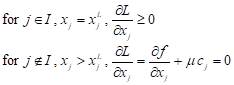 | (6) |
From Eq. (6) we have
| j Î I : xj = xjL |
j Ï I :
 | (7) |
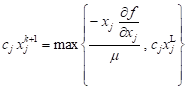
Substituting Eq. (7) into cT x = c0 gives an expression for m, which when substituted back into Eq. (7) gives
| j Î I : xj = xjL |
| j Ï I :
| (8) |
where
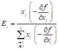 | (9) |
A starting point x0 > xL is used which may be feasible or infeasible with respect to the constraint. We use the fixed-point recurrence relation or ‘re-sizing’ formula:
| j Î I : xj = xjL |
| j Ï I : | (10) |
As per Eq. (1), we use for j Ï I
| (0,1) (11a) |
Or as per Eq. (2) we use for j Ï I
| (11b) |
Basic steps are given in the algorithm below.
3.3. Algorithm steps
Input Data:
x0, xL, w (or p),
gmax, move limit ![]() , Iteration limit,
tolabs, tolrel
, Iteration limit,
tolabs, tolrel
Set initial active set I0 = {null set}
Typical Iteration:
i. Evaluate
derivatives ![]() and then evaluate c, c0,
Ej.
and then evaluate c, c0,
Ej.
ii. Compute xtrial º xk+1 from Eq. (11a) or (11b).
iii.
Reset
xk+1 to satisfy move limits based on ![]() as well as to satisfy the bounds.
as well as to satisfy the bounds.
iv.
Based
on xk+1, update active set from Ik
to Ik+1. A free variable that has reached a bound
is included in the active set based on whether ![]() for
each
for
each ![]() . Also, variables in Ik
are tested if they should become free.
. Also, variables in Ik
are tested if they should become free.
v. Stopping criteria is based on (i) iteration limit (= number of function calls), (ii) based on whether
which should hold for, say, 5 consecutive iterations.
3.4. Extensions of the algorithm
The aforementioned fixed-point algorithm can be applied to problems which are extensions to problem (3) as discussed below.
If the objective is to minimize f where
![]() , subject to
, subject to
g(x) £ 0 where ![]() , then we define reciprocal variables yi
= 1/xi,
i = 1,...,n. Defining f (x) ® f (1/y)
º f new(y) and similarly gnew(y),
we obtain the problem:
, then we define reciprocal variables yi
= 1/xi,
i = 1,...,n. Defining f (x) ® f (1/y)
º f new(y) and similarly gnew(y),
we obtain the problem:
|
subject to gnew(y) £ 0, and y > 0
The switch in the signs of the derivatives allows the algorithm to be applied. For example, the algorithm can be applied to minimize the compliance subject to a mass limit, or to minimize the mass subject to a compliance limit with reciprocal variables.
Upper bounds are present in some problems. In
topology optimization, for
example, the bounds 0 £ xi £ 1 are imposed on the pseudo densities.
The observation made in Section 4 is generalized, viz. ![]() now
represents the available resource after accounting for variables at
their bounds. If a variable xi º q represents
an angle and crosses zero as
now
represents the available resource after accounting for variables at
their bounds. If a variable xi º q represents
an angle and crosses zero as ![]() , it can be
substituted by
, it can be
substituted by ![]() .
.
3.5. Physical interpretation of variable update formula
Importantly, the fixed-point iteration
variable update in Eq. (10) can be physically interpreted as follows. Firstly,
the derivative ![]() has often been termed a
‘sensitivity coefficient’ since it represents, to within a linear
approximation, the change in f due to a unit change in xj.
Similarly, the term
has often been termed a
‘sensitivity coefficient’ since it represents, to within a linear
approximation, the change in f due to a unit change in xj.
Similarly, the term 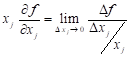 represents the change in f
due to a unit percentage change in xj within a linear
approximation. Thus, as x ® x*, the contribution of the
jth term (cj xj) in the constraint
represents the change in f
due to a unit percentage change in xj within a linear
approximation. Thus, as x ® x*, the contribution of the
jth term (cj xj) in the constraint
| c1 x1 + c2 x2 + ... + ( cj xj ) + ... + cn xn = c0 |
is ‘strengthened’ or
‘trimmed’ based on the relative impact or ‘relative return on investment’ the
variable has on the objective. In structural optimization, this update is
referred to as a ‘re-sizing’ since {xj} refer to member
sizes. Here, the contribution to the literature is that a physical
interpretation has been provided with general functions f and g,
as opposed to specific functions pertaining to structural optimization
applications. Alternatively, dividing through by c0, we may
interpret this as splitting unity into different parts, each part reflecting
the impact on the objective. Lastly ![]() represents the
available resource after accounting for variables at their bounds. Thus, the
variable updates for xj only compete for the resource that is
available. The resizing of variables can thus be expressed as “re-allocate term
(ci xi) = (fractional % reduction in objective) x
(available resource)”. Interestingly, the term
represents the
available resource after accounting for variables at their bounds. Thus, the
variable updates for xj only compete for the resource that is
available. The resizing of variables can thus be expressed as “re-allocate term
(ci xi) = (fractional % reduction in objective) x
(available resource)”. Interestingly, the term ![]() has
only the units of f and is independent of the units of xj.
Also, the iterations are driven by sensitivity only whereas in NLP based
descent methods, the function f is also monitored during the line
search phase.
has
only the units of f and is independent of the units of xj.
Also, the iterations are driven by sensitivity only whereas in NLP based
descent methods, the function f is also monitored during the line
search phase.
4. Applications
4.1. Searching for a missing vessel
Consider the problem of searching for a lost object where it is to be determined how resource b, measured in time units, must be spent to find, with the largest probability, an object among n subdivisions of the area [9]:
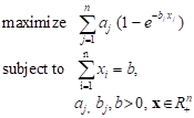 |
Defining ![]() for
minimization, we have
for
minimization, we have ![]() , and derivative of the
constraint function g ≤ 0 is 1. Further, variables are positive.
The fixed-point algorithm can thus be applied.
, and derivative of the
constraint function g ≤ 0 is 1. Further, variables are positive.
The fixed-point algorithm can thus be applied.
4.2. Optimum allocation in stratified sampling
Consider the problem determining an average of a certain quantity among a large population M. The population is stratified into n strata each having a population Mj with the number of samples chosen xj. The total sample is to be allocated to the strata to obtain a minimum variance of the global estimate [9]:
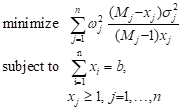 |
where ![]() , s 2 is
an appropriate estimate of the variance .in each strata, b is the total
sample size. We have
, s 2 is
an appropriate estimate of the variance .in each strata, b is the total
sample size. We have ![]() and derivative of the
constraint function g ≤ 0 is 1. Further, variables are positive.
The fixed-point algorithm can thus be applied.
and derivative of the
constraint function g ≤ 0 is 1. Further, variables are positive.
The fixed-point algorithm can thus be applied.
4.3. Structural optimization for minimum compliance
The problem of allocating material within a
structural domain to minimize compliance (i.e. maximize stiffness) satisfies
the assumption ![]() required to use the fixed-point algorithm. Specifically, f
(x) = FTU, with K(x) U = F.
Here, K = global stiffness, U = global displacement, F =
global force, and x represents either a cross-sectional area or element
density. Using the adjoint method [13], it can be shown that if element
stiffness matrix
required to use the fixed-point algorithm. Specifically, f
(x) = FTU, with K(x) U = F.
Here, K = global stiffness, U = global displacement, F =
global force, and x represents either a cross-sectional area or element
density. Using the adjoint method [13], it can be shown that if element
stiffness matrix ![]() with the parameter r
> 0, then
with the parameter r
> 0, then ![]() where ei = qTkq is the element strain energy. Note
that q = the element displacement vector and k = the element
stiffness matrix. Since ei ³ 0 owing to k being positive semi-definite, we have
where ei = qTkq is the element strain energy. Note
that q = the element displacement vector and k = the element
stiffness matrix. Since ei ³ 0 owing to k being positive semi-definite, we have ![]() . Further, the assumption
. Further, the assumption ![]() readily follows when g
represents the total volume of material. Further, in view of
readily follows when g
represents the total volume of material. Further, in view of ![]() , the fraction Ej in
(9) takes the form
, the fraction Ej in
(9) takes the form
 | (13) |
That is, variable update or re-sizing is governed by the energy in the jth element as a fraction of the total energy. Thus, many references exist in structural optimization to energy based optimality criteria methods, which are shown here as special cases stemming from a general formula.
4.4. Real time allocation of resources
In view of the assumptions behind this algorithm, it can be expected to be useful in allocating fixed amount of resources relating to security. This follows from the assumption that more security than needed in certain areas will not be harmful. Similarly, allocating fixed amount of funds to school districts is a possible application. Since the algorithm is fast, a dynamic allocation is possible based on say 30-day moving averages of the data. These applications need to be explored.
5. Numerical examples
Examples are presented to show that the algorithm is far superior to a general nonlinear programming method for problems that satisfy Assumptions 3.1 and 3.2. The fixed-point algorithm is compared to MATLAB’s constrained optimizers (sequential quadratic programming and interior point optimizers under ‘fmincon’).
5.1. Cantilever beam
Consider the simple problem of allocating material to minimize the tip deflection of a cantilever beam with two length segments, with certain assumed problem data:
| minimize |
| subject to 2 x1 + x2 £ 1 |
| x > 0 |
From Eq. (9), ![]() .
The recurrence formula in Eq. (11a) becomes
.
The recurrence formula in Eq. (11a) becomes
where {ci} = [2 1], c0 = 1. The optimum is x* = [0.426, 0.169]. Based on Theorem 2.1, it can be readily shown that the fixed-point iteration converges for w Î(0,1).
5.2. Searching for a missing vessel
Table 1
Searching for a missing vessel
|
N |
NFE1 as per Fixed-point algorithm2 |
NFE as per NLP algorithm2 |
f *_fixed-point, f *_NLP |
|
10 |
37 |
209 |
‒2.338, ‒2.339 |
|
100 |
67 |
4.041 |
‒5.733, ‒5.750 |
|
1003 |
93 |
20,0213 |
‒9.378, ‒9.240 |
1 NFE = Number of Function Evaluations
2 max. constraint violation = 0.001, max NFE = 100, in fixed-point code
3 NLP took 19 iterations, and 20,021 function calls
5.3. Randomized test problem
A set of randomized test problems of the form:
| minimize f (x) = |
| subject to g1
(x) º |
| 0 < xL £ x £ xU |
with the restriction that all
coefficients ![]() > 0,
> 0, ![]() ,
, ![]() . Note that
. Note that
![]() = coefficient of the kth
function, ith term, while ak i j = exponent
corresponding to the kth function, ith term, and jth
variable. Derivatives are calculated analytically.
= coefficient of the kth
function, ith term, while ak i j = exponent
corresponding to the kth function, ith term, and jth
variable. Derivatives are calculated analytically.
Data: xL =
10‒6, xU = 1, ![]() ,
, ![]() ,
, ![]() ,
, ![]() ,
t0 = tk = 8, x0 = 0.5. To
ensure that the constraint is active,
,
t0 = tk = 8, x0 = 0.5. To
ensure that the constraint is active, ![]() .
.
Table 2 shows results for various random generated trials. The fixed-point iteration method far outperforms the NLP routine for the class of problems considered. Total computation in NLP methods increase with n while fixed-point iteration methods are insensitive to it, as also noted in the structural optimization literature.
Table 2
Randomized test problem
|
n |
NFE4 as per Fixed-point algorithm1 |
NFE as per NLP algorithm2 |
f *_fixed-point / f *_NLP 2 |
|
10 |
50 |
363 |
1.027 |
|
20 |
50 |
1,131 |
1.030 |
|
403 |
50 |
3,008 |
1.003 |
1 fixed value
2 averaged over 5 random trials
3 larger values of n cannot be solved in reasonable time by the NLP routine
4 NFE = Number of Function Evaluations
6. Conclusions
In this paper, an optimality criteria based fixed-point iteration is developed for a class of nonlinear programming problems. The class of problems require that the variables are positive, derivatives of f are negative, and derivatives of gj are positive. Certain extensions of this subclass of problems have been given. Hitherto, fixed-point methods were only developed in a problem-specific manner in the field of structural optimization. Convergence aspects are discussed. The fixed-point iteration algorithms to be found in the structural optimization literature, albeit targeting more general problems than considered here, are presented without clearly stating assumptions under which convergence may be achieved, and in fact, have been observed to not converge in certain situations. Moreover, these have been developed for problem specific applications in the structural optimization and have not targeted general functions f and gj even within a subspace of functions. Importantly, the fixed-point update, within this general context, is given physical significance in this paper.
Results show that for the subclass of problems considered, fixed-point iterations far outperform an NLP method. This is a general result because the fixed-point iteration method does not involve line search, a main step in NLP methods, which requires computationally expensive multiple function evaluations, even with the use of approximations. A fixed-point algorithm is insensitive to n whereas in NLP methods, the number of iterations increase significantly with n. In the algorithm presented, the value of w (or p) requires, at most, a one-time adjustment based on a simple rule, viz. if oscillations in the maximum constraint violation are noticed during the iterations, then w is reduced (or p is increased); a smaller value of w than that needed also works except that more iterations are needed, as there is more emphasis on the previous point. A default value of w = 0.25 has worked well on the examples here. New applications need to be explored for using the algorithm.
References
[1] Venkayya V.B., Design of optimum structures, Computers and Structures 1971, 1, 265-309.
[2] Berke L., An efficient approach to the minimum weight design of deflection limited structures, AFFD1-TM-70-4-FDTR, Flight Dynamics Laboratory, Wright Patterson AFB, OH 1970.
[3] Khot N.S., Berke L., Venkayya V.B., Comparison of optimality criteria algorithms for minimum weight design of structures, AIAA Journal 1979, 17(2), 182-190.
[4] Dobbs M.W., Nelson R.B., Application of optimality criteria to automated structural design, AIAA Journal 1975, 14(10), 1436-1443.
[5] Khan M.R., Willmert K.D., Thornton W.A., Optimality criterion method for large-scale structures, AIAA Journal 1979, 17(7), 753-761.
[6] McGee O.G., Phan K.F., A robust optimality criteria procedure for cross-sectional optimization of frame structures with multiple frequency limits, Computers and Structures 1991, 38(5/6), 485- -500.
[7] Yin L., Yang W., Optimality criteria method for topology optimization under multiple constraints, Computers and Structures 2001, 79, 1839-1850.
[8] Belegundu A.D., A general optimality criteria algorithm for a class of engineering optimization problems, Engineering Optimization 2015, 47(5), 674-688.
[9] Patriksson M., A survey on the continuous nonlinear resource allocation problem, European Journal of Operational Research 2008, 185(1), 1-46.
[10] Jose J.A., Klein C.A., A note on multi-item inventory systems with limited capacity, Operations Research Letters 1988, 7(2), 71-75.
[11] Atkinson K.E., An Introduction to Numerical Analysis, John Wiley, 1978.
[12] Bryant V., Metric Spaces: Iteration and Application, Cambridge University Press, 1985.
[13] Belegundu A.D., Chandrupatla T.R., Optimization Concepts and Applications in Engineering, 2nd edition, Cambridge University Press, 2011.