Vibration of the bridge under moving singular loads - theoretical formulation and numerical solution
Marek Szafrański
Journal of Applied Mathematics and Computational Mechanics |
 Download Full Text |
VIBRATION OF THE BRIDGE UNDER MOVING SINGULAR LOADS - THEORETICAL FORMULATION AND NUMERICAL SOLUTION
Marek Szafrański
Faculty of Civil and Environmental
Engineering, Gdansk University of Technology
Gdańsk, Poland
mszafran@pg.gda.pl
Abstract. The paper presents the results of the numerical analysis of a simple vehicle passing over a simply supported bridge span. The bridge is modelled by an Euler-Bernoulli beam. The vehicle is modelled as a linear, visco-elastic oscillator, moving at a constant speed. The system is described by a set of differential equations of motion and solved numerically using the Runge-Kutta algorithm. The results are compared with the solution obtained in commercial FEM software using the Newmark-b method. The parameters of the system are taken from the existing bridge span and from the existing railway vehicle. Simulations are also performed with a concentrated force model of the vehicle.
Keywords: railway bridge, railway load, structure dynamics, bridge-vehicle interaction, differential equations, numerical analysis
1. Introduction
Dynamic analysis of the bridge-vehicle interaction is an important part of design and research work, particularly for high-speed railways. A moving vehicle induces vibration of a bridge span. The bridge in turn affects the vibration of the vehicle. Thus, we have a complex, mutually coupled dynamic system, whose exact analysis is very complicated. The higher the train speed, the greater the dynamic impact to the bridge. A bridge-vehicle interaction analysis requires the dynamic model of the vehicle. In the design practice, the dynamic effects of loads are simplified [1]. A series of concentrated force models are commonly used.
The paper deals with the problem of a linear, single-mass oscillator moving over a simply supported beam. The oscillator can represent a simple vehicle and the beam can simulate a bridge span. The system is described by differential equations of motion. A mathematical formulation and numerical solution is presented. Two numerical methods are used and compared: the Runge-Kutta method of the fourth row and the Newmark-b method. The parameters of the system are taken from the existing bridge (a temporary steel span of 30 m long) and from the existing railway vehicle (EN57 traction unit). The vibrations of the midpoint of the beam as well as the mass of the oscillator are concerned.
The model is shown in Figure 1. The oscillator consists of the mass M (vehicle body), the spring k and the damper h (vehicle suspension) and moves with a constant speed v. The beam has a constant stiffness EI. The unit weight of the beam is m and the damping factor is c. Displacements w(x,t) and u(t) correspond to the beam and to the vehicle respectively.
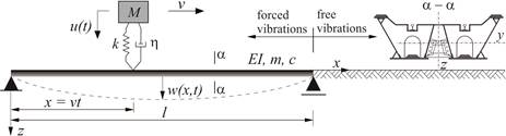
Fig. 1. A model of a single-mass oscillator moving over a simply supported beam
2. Formulation of the problem
A typical problem of a linear dynamics of a discrete, multi degree of freedom (MDOF) system is described by a second order differential equation of motion:
with
initial conditions ![]() . Matrices M, C, K
are the mass, damping and stiffness matrices respectively, P(t)
is an external force vector and
. Matrices M, C, K
are the mass, damping and stiffness matrices respectively, P(t)
is an external force vector and ![]() are the displacement,
velocity and acceleration vectors, respectively. Equation can be formulated using the d’Alembert principle, the Hamilton’s principle or the Lagrange equation of second order. Details can be found in
e.g. [2].
are the displacement,
velocity and acceleration vectors, respectively. Equation can be formulated using the d’Alembert principle, the Hamilton’s principle or the Lagrange equation of second order. Details can be found in
e.g. [2].
For the purpose of this paper, a theoretical formulation of equations of motion was made on the basis of [3]. In the reference, the solution was provided using the Bubnov-Galerkin method. Basic assumptions are as follows:
a) only the vertical displacements are possible,
b) the system is linear and time invariant (LTI system),
c) the deflection of the beam is described by the sine function and only the mid-point of the beam is concerned,
d) the reference level for the vibration of the oscillator is the static equilibrium of the mass: ustat = Mg/k,
e) the oscillator is in full contact with the beam (no separation is possible).
2.1. Force vibration of the oscillator-beam system
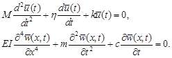
According to aforementioned assumptions and designations depicted in Figure 1, the equation of motion of the oscillator becomes:
where x = vt. The equation of motion of the beam can be written as:
where d(x – vt) is the shifted Dirac delta function for x0 = vt and F(t) is the dynamic force, transmitted between the oscillator and the beam (interaction force). F(t) can be easily obtained from the oscillator equilibrium as follows (Fig. 2):
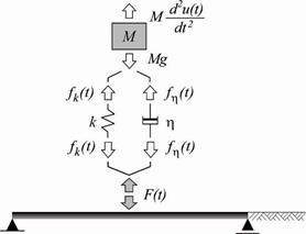
Fig. 2. Forces acting on the elements of the oscillator (vertical motion only)
According to the assumption that the deflection shape of the beam is described by a sine function, the function w(x,t) can be expressed as:
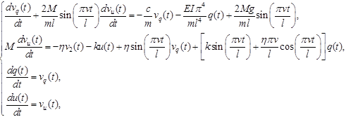
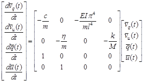
with zero boundary conditions w(0,t) = 0 and w(l,t) = 0. The variable q(t) is a Lagrange coordinate, which describes the displacement in time of the beam. Putting into and and making transformations provided in [3], we finally obtain the system of equations, which describes the vibrations of a coupled oscillator-beam system:
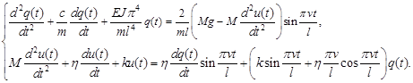 |
The unknown functions u(t) and q(t) can only be numerically determined. The initial conditions are as follows:
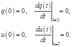 |
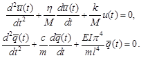
2.2. Free vibrations of the oscillator and the beam
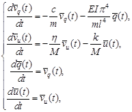
Since the oscillator passed over the beam, both systems perform free vibrations. In this case, the equations for the oscillator and for the beam become:
 |
These are the homogeneous equations with constant coefficients. Unknowns
![]() and
and ![]() are the free response
functions of the beam and of the oscillator respectively. Assuming the solution
of the second of equations as:
are the free response
functions of the beam and of the oscillator respectively. Assuming the solution
of the second of equations as:
we obtain:
 |
The general integral can be derived as follows:
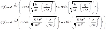 |
where A, B, C, D are
the constants to be determined. Each of the above solutions represent free
responses in time of a single degree of freedom (SDOF) systems with
under-critical damping (see for example ref. [2]). At the moment of time the
oscillator leaves the beam (t = t1), the functions ![]() and
and ![]() and
its first derivatives must be equal. The same applies to the functions
and
its first derivatives must be equal. The same applies to the functions ![]() and
and ![]() . So
in order to determine the constants A, B, C and D, the following initial
conditions can be applied:
. So
in order to determine the constants A, B, C and D, the following initial
conditions can be applied:
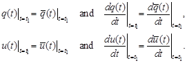 |
Because of , constants A, B, C and D can only be numerically determined.
3. Numerical solution methods
Two numerical methods were used: the Runge-Kutta (R-K) and the Newmark-b method. The R-K method was applied to the equations and and was programmed in MATLAB (ode45 solver was used). The Newmark method allows for direct integration of equation and is implemented in much engineering software of dynamic analysis of structures e.g. in SOFiSTiK FEM software.
3.1. Runge-Kutta method
The group of Runge-Kutta methods allow for a numerical solution of equations in the form of [4]:
Before using the R-K method, equations and should be converted to an equivalent, 1st order form. It can be done using the substitution:
which leads to a system of four equations:
 |
or in a matrix form:
where:
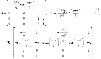 |
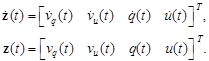 |
Denoting K = A–1B and L = A–1C, system of equations can be written as:
A similar transformation can be performed for the equation . Substitution:
gives the system of four equations:
 |
or in a matrix form:
 , , |
The equation is a linear, first order differential equation with variable coefficients (matrices K and L depend on time t). The set of equations in turn, consists of a linear, first order differential equations with constant coefficients. The forms of both equations are in accordance with the equation , so they can be solved numerically using R-K method.
3.2. Newmark-b method
The method allows for the direct integration of equation , written in the discrete time form:
where un+1 = u(tn+1), tn+1 = tn + Δt and Δt - time step. We are looking
for the solu-
tion at the time step tn+1 (vectors ![]() ),
having known the solution at the time step tn (vectors
),
having known the solution at the time step tn (vectors ![]() ). At
first, a certain type of acceleration variation during an interval
). At
first, a certain type of acceleration variation during an interval ![]() should be assumed [2]. Then, a variation of
velocity and displacement can be derived. In 1959 N.M. Newmark [5]
published the general formula for velocity and displacement vectors as:
should be assumed [2]. Then, a variation of
velocity and displacement can be derived. In 1959 N.M. Newmark [5]
published the general formula for velocity and displacement vectors as:
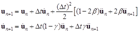 , , |
where b and g are the Newmark parameters. Specializing b and g we obtain the special cases of the method, eg. an average acceleration method (b = 1/4 and g = 1/2), a linear acceleration method (b = 1/6 and g = 1/2). In practice b = 1/4 and g = 1/2 are usually assumed, for which the method is unconditionally stable [2].
Following the transformation presented in [6], from 1 one can obtain:
Putting into 2 gives:
Putting and into , we finally obtain:
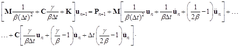 |
From we can calculate the unknown displacement vector un+1 using the
solution in the time step tn (actual
configuration). Then, using and we can calculate the
unknown acceleration and velocity vectors, eg. ![]() and
and ![]() .
.
A detail algorithm and stability discussion of the Newmark-b method can be found in aforementioned references, eg. [2, 5, 6].
4. Numerical simulations
A temporary railway span of 30 m long was adopted as the bridge (Fig. 3). The model of the oscillator was defined on the basis of half of EN57 carriage (Fig. 4).
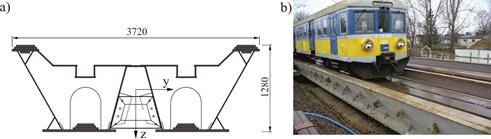
Fig. 3. A considered bridge span: a) a scheme of the cross-section, b) the span in service
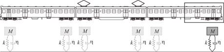
Fig. 4. A scheme of EN57 train
A SOFiSTiK FEM model of the system is shown in Figure 5. The bridge is mod- eled as a simply supported beam. The model is discretized on 61 nodes and 60 beam elements. Each element has 12 DOFS (3 rotations and 3 translations on each node). Because of the 3D model, a rotational degree of freedom (mx) of one support node was blocked additionally to avoid the global instability of the system. Physical parameters of the bridge and of the vehicle were identified in [7]. An Eigensystem Realization Algorithm was used [8]. The parameters are summarized in Table 1.
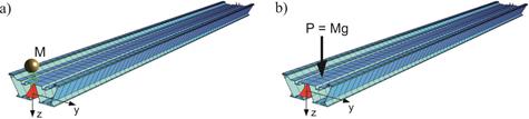
Fig. 5. The FEM model of the system (SOFiSTiK): a) a single mass oscillator model of the vehicle, b) a concentrated force model of the vehicle
Table 1
Physical parameters of the vehicle and of the bridge span
|
Bridge span |
Vehicle |
||
|
Young modulus E [GPa] |
205 |
Mass M [t] |
17.00 |
|
Cross-section A [m2] |
0.3168 |
1st mode frequency fv [Hz] |
2.029 |
|
Moment of inertia Jy [m4] |
0.08143 |
1st mode damping xv [–] |
0.0479 |
|
Unit mass m [t/m] |
2.971 |
Stiffness k [kN/m] |
2762.95 |
|
1st mode frequency fb [Hz] |
4.07 |
Damping coefficient hv [kNs/m] |
20.762 |
|
1st mode damping xb [–] |
0.0117 |
|
|
|
Damping coefficient cb [kNs/m] |
1.744 |
|
|
The damping coefficient of the beam was calculated as cb = xb cbkr = xb 4p m fb , where cbkr is the critical damping of the beam. Similarly, the damping coefficient of the oscillator was calculated as hv = xvxvkr = xv4pMfv . The time step was assumed as Δt = 0.002 s. This value is enough for the stability of both methods.
Figures 6-10 show the results. The vibration of the midpoint of the beam as well as the mass of the oscillator are presented. For 5 kph (“quasi-static” case, Fig. 6), the maximum displacement of the beam and of the oscillator equals the static displacement of the beam: wst = Mgl3/48EI = 5.62∙10–3 m, where g is the acceleration of gravity.
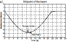
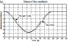
Fig. 6. Vibration of the bridge span (a) and of the vehicle (b) for the velocity of 5 kph
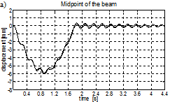
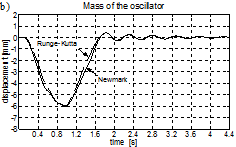
Fig. 7. Vibration of the bridge span (a) and of the vehicle (b) for the velocity of 60 kph
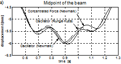
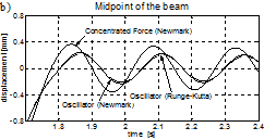
Fig. 8. Vibration of the bridge span for the velocity of 60 kph: a) time interval 0.5÷1.3 s (maximum displacement), b) time interval 1.7÷2.4 s (free response)
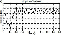
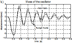
Fig. 9. Vibration of the bridge span (a) and of the vehicle (b) for the velocity of 160 kph
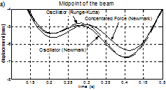
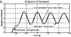
Fig. 10. Vibration of the bridge span for the velocity of 160 kph: a) time interval 0.1÷0.5 s (maximum displacement), b) time interval 0.4÷1.6 s (free response)
5. Conclusions
An application of differential equations and two numerical methods of solution in bridge dynamics is presented. The problem of a linear, single-mass oscillator moving over a simply supported beam is discussed. The physical parameters of the model were taken from the existing bridge span and the existing railway vehicle. A vertical motion of the midpoint of the beam as well as the mass of the oscillator is concerned, so a whole bridge-vehicle system is a 2-DOFs system.
Both numerical solutions (eg. the Runge-Kutta and the Newmark-b solution) are similar. A slight difference can be seen in the oscillator free response amplitudes for the velocity of 160 kph (see Fig. 9b). The higher the speed, the greater the vibration of the bridge and of the vehicle’s body, both of the forced and the free response range. The solution for a concentrated force model of the vehicle is also presented. Some differences in comparison with the oscillator model of a vehicle can be seen, as far as the amplitude and phase of the bridge vibration are concerned (see Figs. 8 and 10). This is because the ‘concentrated force’ formulation omits the inertial terms of moving mass. Moreover, due to the lack of suspension, the dynamic bridge-vehicle interaction effects are not taken into account. It should be noted, however, that the differences are not large. From the technical point of view (eg. for the design practice), the ‘concentrated force’ model is safe and does not overestimate the results at the same time (for the conditions considered in this paper).
It should be finally said that both models of vehicle adopted in this paper differ from an actual railway loading. Single load models are valid only for short spans, carrying a single bogie or even a single wheelset. A more accurate analysis of long span bridges requires considering moving load series, spaced in bogies or wheelset distances [9, 10]. A more advanced analysis, which takes into account 2D or 3D models of vehicles with two levels of suspension, is proposed by Klasztorny [11]. Because of a complex mathematical formulation of these problems, the direct integration Newmark-b method (rather than R-K methods) is commonly used for a numerical solution.
References
[1] Żółtowski K., Kozakiewicz A., Romaszkiewicz T., Szafrański M., Madaj A., Falkiewicz R., Raduszkiewicz T., Redzimski K., Przebudowa mostu kolejowego przez rzekę Pilicę z przystosowaniem do dużych prędkości, Archiwum Instytutu Inżynierii Lądowej 8/2010, XX Seminarium „Współczesne Metody Wzmacniania i Przebudowy Mostów”, Poznań 2010.
[2] Lewandowski R., Dynamika konstrukcji budowlanych, Wydawnictwo Politechniki Poznańskiej, Poznań 2006.
[3] Szcześniak W., Ataman M., Zbiciak A., Drgania belki sprężystej wywołane ruchomym, liniowym oscylatorem jednomasowym, Drogi i Mosty 2002, 2.
[4] Collatz L., Metody numeryczne rozwiązywania równań różniczkowych, PWN, Warszawa 1960.
[5] Newmark N.M., A method of computation for structural dynamics, Journal of Engineering Mechanics, ASCE 1959, 85 (EM3), 67-94.
[6] Lubowiecka I., Całkowanie nieliniowych dynamicznych równań ruchu w mechanice konstrukcji, Dynamika powłok sprężystych, Rozprawa doktorska, Wydział Inżynierii Lądowej, Politechnika Gdańska, Gdańsk 2002.
[7] Szafrański M., Oddziaływania taboru na mosty kolejowe przy zmiennych parametrach ruchu, Rozprawa doktorska, Politechnika Gdańska, Gdańsk 2014.
[8] Juang J.N., Pappa R.S., An eigensystem realization algorithm for modal parameter identification and model reduction, Journal of Guidance, Control and Dynamics 1985, 8(5), 620-627.
[9] Klasztorny M., Analiza drgań belki mostowej przenoszącej jednorodny strumień obciążeń ruchomych, Archiwum Inżynierii Lądowej, 36(3), PWN, Warszawa 1990.
[10] Li J., Su M., The resonant vibration for a simply supported girder bridge under high-speed trains, Journal of Sounds and Vibration 1999, 224(5).
[11] Klasztorny M., Dynamika mostów belkowych obciążonych pociągami szybkobieżnymi, WNT, Warszawa 2005.