Asymmetric detrended fluctuation analysis reveals asymmetry in the RR intervals time series
Dawid Mieszkowski
,Marcin Kośmider
,Tomasz Krauze
,Przemysław Guzik
,Jarosław Piskorski
Journal of Applied Mathematics and Computational Mechanics |
 Download Full Text |
ASYMMETRIC DETRENDED FLUCTUATION ANALYSIS REVEALS ASYMMETRY IN THE RR INTERVALS TIME SERIES
Dawid Mieszkowski 1, Marcin Kośmider 1, Tomasz Krauze 2 Przemysław Guzik 2, Jarosław Piskorski 1
1 Institute
of Physics, University of Zielona Gora
Zielona Góra, Poland
2 Department of Cardiology - Intensive Therapy, University of
Medical Sciences
Poznań, Poland
dawid.mieszkowski@gmail.com, kosmo@codelab.pl, tomaszkrauze@wp.pl
pguzik@ptkardio.pl, jaropis@zg.home.pl
Abstract. In
this paper we apply the Asymmetric Detrended Fluctuation Analysis to the RR
intervals time series. The mathematical background of the ADFA method is
discussed in the context of heart rate variability and heart rate asymmetry. We
calculate the ![]() and
and ![]() ADFA scaling exponents
for 100 RR intervals time series recorded in a group of healthy
volunteers (20-40 years of age) with the use of the local ADFA. It is found
that on average
ADFA scaling exponents
for 100 RR intervals time series recorded in a group of healthy
volunteers (20-40 years of age) with the use of the local ADFA. It is found
that on average ![]() , and that locally
, and that locally ![]() dominates most of the
time over
dominates most of the
time over ![]() - both results are highly statistically
significant.
- both results are highly statistically
significant.
Keywords: scaling exponents, random walk, detrended fluctuation analysis, heart rate variability, heart rate asymmetry
1. Introduction
The RR intervals time series, which is the time series of time intervals between successive R-waves (see Fig. 1), is perhaps one of the most often studied signals of physiological origin. It is easily obtainable and its structure lends itself well to various existing time-series analysis methods.
The most often used approach to RR intervals time series is the heart rate variability (HRV) analysis which explores the changes of this series in time and tries to relate the results to various physiological or pathological states [1].
The RR intervals time series is nonstationary in the sense that it does not have well-defined moments [1]. Consequently, many of the HRV methods can only be related to the specific analysed series since quantities like mean or variance cannot be related to the underlying generating process.
In recent years there have been many attempts to deal with the nonstationarity problem - one of them is the detrended fluctuation analysis (DFA) [2, 3], another one is the Heart Rate Asymmetry (HRA) analysis [4, 5]. The former analyses the correlational structure of the noise remaining after detrending the time series, the latter concentrates on the quantification and qualification of the systematic differences between heart rate accelerations and decelerations in the variance, structure and complexity spaces.
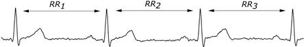
Fig. 1. Formation of the RR intervals time series as the sequence of time distances between consecutive heart beats (distances between the consecutive R-waves)
A recent method of Asymmetric Detrended Fluctuation Analysis (ADFA) seems to be capable of summarizing both the correlational structure of the RR-intervals time series and the differences between accelerating and decelerating segments [6, 7].
The aim of this paper is to apply the ADFA technique to the RR intervals time series in order to see whether this asymmetric technique also reveals the asymmetry inherent in the heart rate.
2. Detrended fluctuation analysis
The method of detrended fluctuation analysis studies the random walk defined on the analysed time series. The basic idea is to calculate the variance of the random walk at a number of scales and study the relationship between the variance and scale. For example, for a random walk defined by a coin flip we have
| (1) |
where ![]() is the number of
steps of length 1 in the random walk [8]. This is an example of a more general type of
statistical property of a time series, namely
is the number of
steps of length 1 in the random walk [8]. This is an example of a more general type of
statistical property of a time series, namely
| (2) |
where ![]() is the universal
critical exponent which is characteristic of a power law observed in
scale-invariant systems [8].
is the universal
critical exponent which is characteristic of a power law observed in
scale-invariant systems [8].
The above analysis can be applied to a number of correlated or uncorrelated types of noise. The RR-intervals time series, however, is non-stationary as it contains trends. The detrended fluctuation analysis aims at defining a “random walk” on this time series by removing these trends and analysing the resulting noise.
This is achieved by defining the root mean square fluctuation of the random walk
|
|
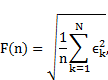
where ![]() is defined as an
integrated and detrended time series as follows.
is defined as an
integrated and detrended time series as follows.
First, let us define the original time series as
| (4) |
i.e. it is a time
series of ![]() consecutive
consecutive ![]() intervals indexed by the number of the cardiac evolutions.
intervals indexed by the number of the cardiac evolutions.
The mean of this time series is different from zero, so the random walk defined on it would contain drift, therefore, before integrating, the mean is subtracted
|
|
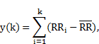
where ![]() is the mean of the
time series [2, 3].
is the mean of the
time series [2, 3].
This integrated time series is divided into
segments of constant length ![]() and
in each segment a straight line is fitted
and
in each segment a straight line is fitted
| (6) |
and finally the fluctuation ![]() used in equation (3)
is defined as
used in equation (3)
is defined as
| (7) |
i.e. the local trends
are removed from the integrated time series [2, 3, 6, 7]. The
![]() and
and ![]() parameters may be fitted with any optimization technique like, for
example, the least squares method.
parameters may be fitted with any optimization technique like, for
example, the least squares method.
![]() defined in equation
(3) is now calculated for all time scales available
in the time series and the power law relationship between this fluctuation and
box size is explored [2, 3]. If
defined in equation
(3) is now calculated for all time scales available
in the time series and the power law relationship between this fluctuation and
box size is explored [2, 3]. If
| (8) |
holds, we may conclude the existence of the power law and, consequently, the existence of long-range correlations in the time series [2, 3, 8].
It is worth noting
that the number of scales necessary for ![]() calculation can be
greatly reduced by using the approach suggested by Peng et al. in [9].
calculation can be
greatly reduced by using the approach suggested by Peng et al. in [9].
The value of the ![]() exponent, often called
scaling exponent, is derived by fitting a straight line to the
exponent, often called
scaling exponent, is derived by fitting a straight line to the ![]() on
on ![]() plot. This exponent is
used to classify the analysed noise [2, 3]:
plot. This exponent is
used to classify the analysed noise [2, 3]:
·
![]() - negative long-range
correlations,
- negative long-range
correlations,
·
![]() - white noise with no
correlations,
- white noise with no
correlations,
·
![]() - positive long-range
correlations,
- positive long-range
correlations,
·
![]() -
- ![]() noise, typical of many
biological time series,
noise, typical of many
biological time series,
·
![]() - positive long-range
correlations which do not follow the power law,
- positive long-range
correlations which do not follow the power law,
·
![]() - red (Brownian)
noise.
- red (Brownian)
noise.
Figure 2 presents the DFA of one of the
recordings used in this paper. It can be seen that the ![]() exponent is consistent
with 1, so it can be concluded that there is
exponent is consistent
with 1, so it can be concluded that there is ![]() noise in the analysed
signal.
noise in the analysed
signal.
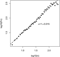
Fig. 2. Example DFA analysis of an RR-intervals time series from a 33 year-old male
3. Asymmetric detrended fluctuation analysis
In recent years there has been a lot of research on the asymmetric properties of the RR intervals time series [4, 5, 10]. The reason for this is the fact that the accelerations and decelerations of heart rate are well-defined physiological processes, even though the specific mechanisms that govern them are very complex. It has been demonstrated that parameters describing the asymmetric behaviour of the RR intervals time series have prognostic value in the sense that the prognosis of the patient, like for instance the probability of surviving the next two years after myocardial infarction, can be informed by analysing the asymmetric parameters [10].
At the same time, for different reasons, the
DFA has been extended to the asymmetric case and the asymmetric detrended
fluctuation analysis (ADFA)
approach was created [6, 7]. The motivation for doing so may be found in
[6, 7]. This modification consists of two steps. First, the time series
are divided into
segments with rising and falling trends (on the basis of the sign of the ![]() statistic - compare
eq. (6)). Then fluctuations on raising and falling trends are defined
separately as
statistic - compare
eq. (6)). Then fluctuations on raising and falling trends are defined
separately as
|
|
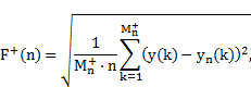
for rising trends, and
|
|
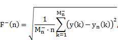
for falling trends. ![]() is the number of boxes
of length
is the number of boxes
of length ![]() with rising/falling
trend, respectively, [7].
with rising/falling
trend, respectively, [7].
Asymmetric scaling exponents are defined as
| (11) |
provided that power law holds [6, 7].
Similarly to the standard DFA, the ![]() exponents are derived
from the plots of
exponents are derived
from the plots of ![]() on
on ![]() [6, 7].
[6, 7].
Another modification concerns the mode of calculating the asymmetric exponents. It is possible to calculate them for the entire recording with RR intervals, however, since the very long trends present in the RR intervals time series can be ascribed to activity or circadian rhythms, which are not part of the autonomic system modulation (they can influence it, though), it seems reasonable to concentrate on shorter scale trends. Another reason is the fact that the acceleration and deceleration runs, which form the basis of one of the more successful approaches to HRA, are observable on a short scale, the longest being the acceleration runs of length approximately 20 beats [5, 10].
A localized version of ADFA was developed in
[7]. It boils down to calculating the ![]() exponents in sliding
or jumping windows, in the original paper the length
of this window was selected to be 100 samples long, and producing two
derivative time series of
exponents in sliding
or jumping windows, in the original paper the length
of this window was selected to be 100 samples long, and producing two
derivative time series of ![]() and
and ![]() .
.
4. Materials and methods
The studied group consisted of 100 healthy volunteers, 45 women, age range 20-40 years. In each subject standard 30-minute, 12-lead ECG was recorded at 1600 Hz. The ECG curves were registered by the analog-digital converter (Porti 5, TMSI, The Netherlands) and saved to the hard disk. The post-processing was carried out with the libRASCH/RASCHlab (v. 0.6.1, Raphael Schneider, Germany). The automatic classification into beats of sinus, ventricular, supraventricular and artifact was verified by an expert who edited the classification as the need arose. The RR intervals with annotations were exported to text files which were further analysed by the in-house software written in python and cython for dynamic ADFA (the git repository for this software with complete code can be found at https://github.com/kosmo76/adfa). The analysis used a 100 long sliding window.
The results were analysed with the use of the R statistical package and programming language. For each recording the average and standard deviation were calculated, and these results were used to calculate the mean and standard deviation weighted by the variances of each recording, according to
|
|

and these values were reported.
After checking for normality of the
distribution of the ![]() , they were used for
the paired t-test for equality of the means. The resulting
, they were used for
the paired t-test for equality of the means. The resulting ![]() time series were also
analysed for the time during which
time series were also
analysed for the time during which ![]() and vice versa. Since
for random data the times should be equal, the binomial test was used to
establish whether any of the above inequalities clearly dominates.
and vice versa. Since
for random data the times should be equal, the binomial test was used to
establish whether any of the above inequalities clearly dominates.
5. Results
The mean value of ![]() was 0.89 ±0.02, the mean
value of
was 0.89 ±0.02, the mean
value of ![]() was 0.98 ±0.02. The
comparison with the paired t-test yields p < 0.0001,
which means that there is a highly statistically significant difference between
was 0.98 ±0.02. The
comparison with the paired t-test yields p < 0.0001,
which means that there is a highly statistically significant difference between
![]() , and
, and ![]() , with
, with ![]() . Both the distribution of the
. Both the distribution of the ![]() values and the paired t-test are illustrated in Figure 3.
values and the paired t-test are illustrated in Figure 3.
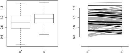
Fig. 3.
Comparison of the ![]() and
and ![]() scaling exponents. The
left panel presents
the boxplots of these exponents, the right panel demonstrates the paired t-test
comparison. The lines connect
scaling exponents. The
left panel presents
the boxplots of these exponents, the right panel demonstrates the paired t-test
comparison. The lines connect ![]() and
and ![]() scaling exponents from
the same
recording - grey corresponds to
scaling exponents from
the same
recording - grey corresponds to ![]() and black to the reversed
inequality
and black to the reversed
inequality
Another way in which the asymmetry can be
observed in ADFA is counting
the time during which ![]() . Overall, of the 100
analysed recordings, in 82 we observed
. Overall, of the 100
analysed recordings, in 82 we observed ![]() , in the remaining ones
the inequality was reversed. It is interesting to note that this result is
similar to the percentages obtained for variance-based asymmetry descriptors
[4]. This result can be analysed with the use of the binomial test: if the time
series was symmetric, there should be no differences between
upward and downward trends, so the proportion should be 0.5 rather than the
observed 0.8. The binomial test shows that the difference between the obtained
result and the symmetric result is highly statistically significant with p < 0.0001.
This analysis is illustrated in Figure 3 above.
, in the remaining ones
the inequality was reversed. It is interesting to note that this result is
similar to the percentages obtained for variance-based asymmetry descriptors
[4]. This result can be analysed with the use of the binomial test: if the time
series was symmetric, there should be no differences between
upward and downward trends, so the proportion should be 0.5 rather than the
observed 0.8. The binomial test shows that the difference between the obtained
result and the symmetric result is highly statistically significant with p < 0.0001.
This analysis is illustrated in Figure 3 above.
6. Conclusions
In the present paper we have applied the ADFA
technique to short, 30-minute long, stationary recordings. We have used the
local version
of ADFA which utilizes jumping, 100-beat
window and calculates the scaling exponents ![]() and
and ![]() for each window, thus creating a derivative,
multivariate time series.
for each window, thus creating a derivative,
multivariate time series.
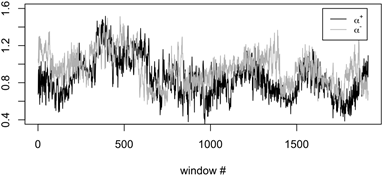
Fig. 4. Example of
the local value of the ![]() and
and ![]() scaling exponents in
one recording.
It is evident that most of the time there is
scaling exponents in
one recording.
It is evident that most of the time there is ![]()
The result obtained was that there is a clear
and easily observable asymmetry
in the correlational structure of the RR intervals time series. We
observed that,
averaged over all the local windows, there is ![]() , and this observation
is highly statistically significant. Also, inequality of the same direction is
observable in the time in which it is fulfilled: in 80% of the recordings, for
the majority
of time, there was
, and this observation
is highly statistically significant. Also, inequality of the same direction is
observable in the time in which it is fulfilled: in 80% of the recordings, for
the majority
of time, there was ![]() . This result is also
highly statistically significant.
. This result is also
highly statistically significant.
HRA was first observed using the variance based descriptors and then expanded upon with the use of the method of accelerations and decelerations runs [4, 5, 10]. The main mechanism in which HRA arises mathematically is the fact that decelerations seem to be more dynamic than accelerations in the sense that fewer steps are needed to decelerate by, say, 50 bpm (beats per minute), than to accelerate by the same amount [5, 10]. The original papers introducing ADFA aimed at describing economic time series [6, 7], in which collapses are much more dynamic than recoveries. It is very possible that the fact that asymmetry is also visible in the RR intervals follows from this similarity between the two types of time series.
One limitation of the method used in the present paper could be raised here. The ADFA practically treats falling and rising trends as if they were coming from two separate time series or two separate processes. In the case of heart rate it is very difficult to say with certainty what caused an acceleration or deceleration. The dynamic balance between the parasympathetic and sympathetic branches of the autonomic nervous system is responsible for the instant changes of heart rate that can be observed in a form of accelerations and decelerations. The widespread belief that it is the parasympathetic branch of the autonomic system which is responsible for decelerations and the sympathetic branch which is responsible for accelerations is only a first approximation and in reality these processes are much more complex.
Nevertheless, ADFA is a new and promising method of exploring the inherent asymmetry of the RR intervals time series. Further studies, both theoretical and data-based are necessary to understand both the mathematical structure of the method and its results when applied to the very important and very complex RR intervals time series.
References
[1] Sassi R., Cerutti S., Lombardi F., Malik M., Huikuri H.V., Peng C.K., Schmidt G., Yamamoto Y., Advances in heart rate variability signal analysis: Joint position statement by the e-Cardiology ESC Working Group and the European Heart Rhythm Association co-endorsed by the Asia Pacific Heart Rhythm Society, Europace 2015, 17, 1341-1353.
[2] Peng C.K., Buldyrev S.V., Havlin S., Simons M., Stanley H.E., Goldberger A.L., Mosaic organization of DNA nucleotides, Phys. Rev. E 1994, 49, 1685-1689.
[3] Peng C.K., Havlin S., Stanley H.E., Goldberger A.L., Quantification of scaling exponents and crossover phenomena in nonstationary heartbeat time series, Chaos 1995, 5, 82-87.
[4] Piskorski J., Guzik P., Geometry of the Poincaré plot of RR intervals and its asymmetry in healthy adults, Physiol. Meas. 2007, 28, 287-300.
[5] Piskorski J., Guzik P., The structure of heart rate asymmetry: deceleration and acceleration runs, Physiol. Meas. 2011, 32, 1011-1023.
[6] Ramirez J.A., Rodrigues E., Echeverria J.C., A DFA approach for assessing asymmetric correlations, Physica A 2009, 388, 2263-2270.
[7] Rivera-Castro M.A., Miranda J.G.V., Cajueiro D.O., Andrade R.F.S., Detecting switching points using asymmetric detrended fluctuation analysis, Physica A 2012, 391, 170-179.
[8] Sethna J.P., Statistical Mechanics: Entropy, Order Parameters and Complexity, Oxford University Press, Oxford 2006.
[9] Goldberger A.L., Amaral L.A.N., Glass L., Hausdor J.M., Ivanov P.Ch., Mark R.G., Mietus J.E., Moody G.B., Peng C.K., Stanley H.E., PhysioBank, Physio-Toolkit, and Physionet: Components of a new research resource for complex physiologic signals, Circulation 2001, 101, e215-e220.
[10] Guzik P., Piskorski J., Barthel P., Bauer A., Müller A., Junk N., Ulm K., Malik M., Schmidt G., Heart rate deceleration runs for postinfarction risk prediction, J. Electrocardiol. 2012, 45, 70-75.