Statistical analysis of mechanical damage in nanopillar arrays with mixed-mode load transfer
Tomasz Derda
Journal of Applied Mathematics and Computational Mechanics |
 Download Full Text |
STATISTICAL ANALYSIS OF MECHANICAL DAMAGE IN NANOPILLAR ARRAYS WITH MIXED-MODE LOAD TRANSFER
Tomasz Derda
Institute of Mathematics, Czestochowa
University of Technology
Czestochowa, Poland
tomasz.derda@im.pcz.pl
Received: 12 July 2017; Accepted: 18 September 2017
Abstract. In the framework of the Fibre Bundle Model we explore the effect of mixed- -mode load transfer in two-dimensional arrays of nanopillars. The mixed-mode load redistribution scheme serves as an interpolation between limiting cases, namely global and local transfer. Two types of loading processes are employed i.e. quasi-static and sudden loading. By varying the weight parameter, we identify two behaviours: the GLS and LLS regime. As a regime indicator we use distribution of critical loads and function fitting probability of system breakdown.
MSC 2010: 82D30, 82D80, 65Z05
Keywords: array of pillars, load transfer rule, probability and statistics, crossover, critical load
1. Introduction
The phenomena of failure and fracture of materials are a complex collection of phenomena in science and engineering. For the reason of the disorder in the materials and their inherent nonuniformity, the failure processes of real materials usually cannot be described by simple linear equations. Therefore, statistical models are widely used to study the fracture and breakdown processes. One of the most important theoretical approaches is the fibre bundle model (FBM) [1-3], which illustrates a stochastic fracture-failure process in disordered materials subjected to external load. The key aspect of the FBM is a load transfer rule which is responsible for the mechanism of redistribution of load carried by the broken fibres (elements) to the intact ones. The load sharing rules can be divided into two extreme classes: global load sharing (GLS) and local load sharing (LLS). In the GLS model, long-range interactions are assumed as all the intact elements equally share a load of a failed element. The LLS model represents short-range interactions - the load from the destroyed element is redistributed only to its nearest intact neighbours. Both of these rules are idealised cases, hence Pradhan et al. [4] proposed the mixed-mode load sharing rule and explored it for one-dimensional case.
In this work, using the mixed-mode FBM, we analyse chosen quantities of damage processes in arrays of vertical nanopillars distributed on a flat substrate. The paper is organised as follows. The model is described in the next section. Then, simulation results are presented and discussed. In the final section our findings are summarised briefly.
2. Model
We consider the system as a set of ![]() longitudinal nanopillars located in the
nodes of the supporting lattice. We analyse only regular arrangements i.e.
hexagonal, square and triangular grids. However, the main interest is devoted
to the square lattice case, which is seen as a set of
longitudinal nanopillars located in the
nodes of the supporting lattice. We analyse only regular arrangements i.e.
hexagonal, square and triangular grids. However, the main interest is devoted
to the square lattice case, which is seen as a set of ![]() pillars
with
pillars
with ![]() being the linear
dimension. If it not specified otherwise, we explore the square lattice case.
being the linear
dimension. If it not specified otherwise, we explore the square lattice case.
Each pillar is characterised by its own
strength threshold to an applied axial load. The existence of defects in actual
materials plays a key role in the mechanical response of materials under load.
Hence, pillar-strength-thresholds ![]() ,
, ![]() are quenched random variables
distributed according to the two-parameter Weibull distribution
are quenched random variables
distributed according to the two-parameter Weibull distribution
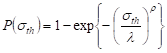 | (1) |
where ![]() is the shape parameter, also known as
the Weibull index, and
is the shape parameter, also known as
the Weibull index, and ![]() is the scale parameter. The
first parameter controls the amount of disorder in the system. In this work we
assume
is the scale parameter. The
first parameter controls the amount of disorder in the system. In this work we
assume ![]() and
and ![]() ,
which means strong disorder.
,
which means strong disorder.
The system is subjected to axial external loading. In the following simulation it is instructive to consider two different, but also equivalent, loading procedures: quasi-static loading and sudden loading (finite force application). For both of these processes the uniform loading is assumed, however, the internal load transfers can cause inhomogeneities in loads of individual pillars.
In the case of quasi-static loading the
external load ![]() is gradually increased up to
the complete failure of the system. Initially the system is unloaded and intact.
Then the load is uniformly increased on all the working pillars just to destroy
the weakest one. Then, the increase of the external load is stopped and the
load from the destroyed pillar is transferred to intact pillars. The load
redistribution may lead to subsequent pillar failures which can provoke the
next failures. A stable state is achieved if the load redistribution does not
cause any failures. In such a situation, the external load has to be increased
again. The above described dynamics is continued until destruction of all
pillars.
is gradually increased up to
the complete failure of the system. Initially the system is unloaded and intact.
Then the load is uniformly increased on all the working pillars just to destroy
the weakest one. Then, the increase of the external load is stopped and the
load from the destroyed pillar is transferred to intact pillars. The load
redistribution may lead to subsequent pillar failures which can provoke the
next failures. A stable state is achieved if the load redistribution does not
cause any failures. In such a situation, the external load has to be increased
again. The above described dynamics is continued until destruction of all
pillars.
Sudden loading of the system is realised by
application of an external force ![]() which is kept
constant during the entire loading process. Due to uniform loading, in the
moment of application of load
which is kept
constant during the entire loading process. Due to uniform loading, in the
moment of application of load ![]() the load per pillar
is
the load per pillar
is ![]() , so all the pillars with strength
thresholds smaller than
, so all the pillars with strength
thresholds smaller than ![]() are immediately
destroyed. Then, the load transfers may lead to the next failures. This
procedure leads to a stable state of the system which is either partially or
fully destroyed. The third possibility is that the system is intact - only if
are immediately
destroyed. Then, the load transfers may lead to the next failures. This
procedure leads to a stable state of the system which is either partially or
fully destroyed. The third possibility is that the system is intact - only if ![]() is not greater than
is not greater than ![]() of the weakest pillar.
of the weakest pillar.
As a load transfer
rule, we apply mixed-mode load sharing with weight parameter ![]() . In this scheme, when a pillar fails, fraction
. In this scheme, when a pillar fails, fraction ![]() of its load is
transferred locally and the rest (
of its load is
transferred locally and the rest (![]() fraction) is distributed globally. Therefore, the mixed-mode load sharing is
an interpolation mechanism between the GLS and LLS –
fraction) is distributed globally. Therefore, the mixed-mode load sharing is
an interpolation mechanism between the GLS and LLS – ![]() corresponds to the GLS rule and
corresponds to the GLS rule and ![]() represents the pure
LLS rule.
represents the pure
LLS rule.
3. Analysis of the simulation results
Based on the model
presented in the previous section, we have developed
program codes for simulation of damage processes in the nanopillar arrays.
Then, we have performed intensive computer simulations. Generally, we study the
behaviour of the model from ![]() up to
up to ![]() with a step of 0.05. Because of
computational time limitations, in some cases we increase step to 0.1.
with a step of 0.05. Because of
computational time limitations, in some cases we increase step to 0.1.
3.1. Quasi-static loading
For the
quasi-static loading, the damage process proceeds in an avalanche-like manner.
Although initial load increases provoke only single pillar failures, further
load increases involve bursts of failures. Such a single failure or a burst of
pillar failures caused by load increase is called an avalanche (![]() ). Application of quasi-
-static loading process ensures obtaining the minimum external load
). Application of quasi-
-static loading process ensures obtaining the minimum external load ![]() that is needed to induce catastrophic
avalanche
that is needed to induce catastrophic
avalanche ![]() which contains all previously
undestroyed pillars. Therefore, we can find the maximum value of applied load
which contains all previously
undestroyed pillars. Therefore, we can find the maximum value of applied load ![]() (total critical load) that can be
supported by the system. The strength of the bundle can be scaled by the system
size, thus giving critical load per pillar
(total critical load) that can be
supported by the system. The strength of the bundle can be scaled by the system
size, thus giving critical load per pillar ![]() .
.
For the GLS rule,
we assume that the support-pillar interface is perfectly rigid, whereas, in the
case of the LLS rule, this support has a certain compliance. Thus, for the GLS
all the intact pillars are under equal load and the geometry of lattice is
irrelevant. This is in contrast to the LLS rule, where load redistribution is localized
and distribution of load is not homogeneous. By increasing ![]() , load transfer changes from pure
long-range (
, load transfer changes from pure
long-range (![]() ) to strictly localized (
) to strictly localized (![]() ). In the following we analyse how it
influences the mean value of critical load
). In the following we analyse how it
influences the mean value of critical load ![]() .
.
It is known from
[5-7] that for the Weibull distributed elements and the GLS rule the mean
critical load ![]() asymptotically tends to:
asymptotically tends to:
| (2) |
Different
behaviour is observed for the LLS scheme - ![]() tends
to zero in the asymptotic limit. We have found that
tends
to zero in the asymptotic limit. We have found that ![]() can
be nicely fitted by the function [8]:
can
be nicely fitted by the function [8]:
| (3) |
with ![]() and
and ![]() .
These values of the parameters were not published yet. Formula (3) concerns
two-dimensional square grids and was originally fitted to systems with
uniformly distributed pillar-strength-thresholds.
.
These values of the parameters were not published yet. Formula (3) concerns
two-dimensional square grids and was originally fitted to systems with
uniformly distributed pillar-strength-thresholds.
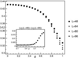
Fig. 1. The mean critical load versus weight
parameter ![]() for different system sizes.
The averages are taken from at least 5000 samples for each presented value. In
the inset we show the results of subtracting
for different system sizes.
The averages are taken from at least 5000 samples for each presented value. In
the inset we show the results of subtracting ![]() for
for ![]() from
from ![]() for
for ![]()
In Figure 1 we
have plotted, for different system sizes, the mean critical load ![]() as a function of weight parameter
as a function of weight parameter ![]() . The function is strictly decreasing -
as
. The function is strictly decreasing -
as ![]() is increased, the load transfer becomes
more and more localised which causes weakening of the system. It is also seen
that for
is increased, the load transfer becomes
more and more localised which causes weakening of the system. It is also seen
that for ![]() values of
values of ![]() are
almost identical irrespective of the system size, and this suggests dominance
of long-range interactions (GLS regime). Then, for higher values of
are
almost identical irrespective of the system size, and this suggests dominance
of long-range interactions (GLS regime). Then, for higher values of ![]() the differences between
the differences between ![]() for presented system sizes noticeably
increase (see inset in Figure 1). From
for presented system sizes noticeably
increase (see inset in Figure 1). From ![]() we
distinctly observe a size-dependent behaviour which is an evidence of LLS
regime dominance. The similar behaviour was reported by Pradhan et al. [4], but
the results are not directly comparable, because their results concern a one-dimensional
model with uniformly distributed strength-thresholds.
we
distinctly observe a size-dependent behaviour which is an evidence of LLS
regime dominance. The similar behaviour was reported by Pradhan et al. [4], but
the results are not directly comparable, because their results concern a one-dimensional
model with uniformly distributed strength-thresholds.
To analyse the
influence of pillar arrangements, we compare the results of ![]() for three regular lattices (see Figure
2). Each lattice is characterised by its own number of nearest neighbours,
namely hexagonal - 3, square - 4 and triangular - 6. In the classical LLS
scheme, as the number of nearest neighbours increases the load from the
destroyed pillar becomes more dispersed and thus leads to a strengthening
of the system. For the LLS the hexagonal system is the weakest, while the
triangular system is the strongest one. The same behaviour is observed for the
mixed-mode (
for three regular lattices (see Figure
2). Each lattice is characterised by its own number of nearest neighbours,
namely hexagonal - 3, square - 4 and triangular - 6. In the classical LLS
scheme, as the number of nearest neighbours increases the load from the
destroyed pillar becomes more dispersed and thus leads to a strengthening
of the system. For the LLS the hexagonal system is the weakest, while the
triangular system is the strongest one. The same behaviour is observed for the
mixed-mode (![]() ) although, for smaller values of
) although, for smaller values of ![]() , the differences are close to 0. From
, the differences are close to 0. From ![]() , the results for hexagonal lattice
start to visibly differ from the results obtained for square and triangular
geometries, while the results for these two geometries are almost equal up to
, the results for hexagonal lattice
start to visibly differ from the results obtained for square and triangular
geometries, while the results for these two geometries are almost equal up to ![]() .
.
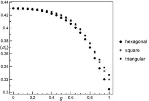
Fig. 2. The mean
critical load as a function of weight parameter ![]() for
different system geometries and
for
different system geometries and ![]() . The averages are
taken from at least 5000 samples for each presented value
. The averages are
taken from at least 5000 samples for each presented value
In our previous
works, we have noticed that for the LLS model the distribution of ![]() can be fitted by three-parameter skew
normal distribution (SND) with
probability density function [9, 10]:
can be fitted by three-parameter skew
normal distribution (SND) with
probability density function [9, 10]:
 | (4) |
and cumulative distribution function (CDF)
| (5) |
where ![]() ,
, ![]() ,
, ![]() are location, scale and shape
parameters, respectively. Function
are location, scale and shape
parameters, respectively. Function![]() represents a
complimentary error function and
represents a
complimentary error function and ![]() is Owen’s T
function.
is Owen’s T
function.
In the case of the
GLS model, distribution of ![]() follows normal
distribution. Skew normal distribution is a generalisation of normal
distribution for non-zero skewness. Therefore, we have fitted distribution of
follows normal
distribution. Skew normal distribution is a generalisation of normal
distribution for non-zero skewness. Therefore, we have fitted distribution of ![]() for the mixed-mode scheme by skew
normal distribution. But first, in Figure 3, we present results of skewness of
for the mixed-mode scheme by skew
normal distribution. But first, in Figure 3, we present results of skewness of ![]() distribution for different values of
distribution for different values of ![]() and chosen system sizes. We can see
that up to
and chosen system sizes. We can see
that up to ![]() distribution of
distribution of ![]() is
approximately symmetric. From
is
approximately symmetric. From ![]() up to
up to ![]() skewness is negative like in the LLS
case and moderate skewness is approached.
skewness is negative like in the LLS
case and moderate skewness is approached.
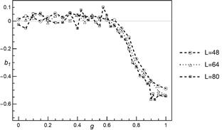
Fig. 3. The skewness of critical load as a
function of weight parameter ![]() for different system
sizes. The results are taken from at least 5000 samples for each presented
value
for different system
sizes. The results are taken from at least 5000 samples for each presented
value
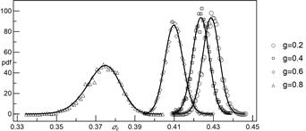
Fig. 4. Empirical probability density
functions of the ![]() in an array of
in an array of ![]() pillars. The solid lines represent
probability density function of skew normally distributed
pillars. The solid lines represent
probability density function of skew normally distributed ![]() with parameters computed from the
samples
with parameters computed from the
samples
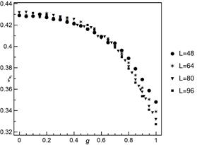
Fig. 5. The location parameter ![]() of skew normal distribution as a
function of
of skew normal distribution as a
function of ![]() for different system sizes
for different system sizes

Fig. 6. The scale parameter ![]() of skew normal distribution as a
function of
of skew normal distribution as a
function of ![]() for different system sizes
for different system sizes
Figure 4
illustrates exemplary empirical probability density functions of ![]() for different values of weight
parameter
for different values of weight
parameter ![]() . Figures 5-7 graphically report fitted
values of parameters of skew normally distributed
. Figures 5-7 graphically report fitted
values of parameters of skew normally distributed ![]() .
Each presented result is based on at least 20,000 independent samples (
.
Each presented result is based on at least 20,000 independent samples (![]() ), 10,000 samples (
), 10,000 samples (![]() ) and 5,000 samples (
) and 5,000 samples (![]() and
and ![]() ). In
Figure 4, two regimes can be noticed. For
). In
Figure 4, two regimes can be noticed. For ![]() we
see three curves similar to each other in terms of dispersion, which is low in
comparison to dispersion for
we
see three curves similar to each other in terms of dispersion, which is low in
comparison to dispersion for ![]() . This observation is
supported by Figure 6, where a noticeable increase of estimated scale parameter
. This observation is
supported by Figure 6, where a noticeable increase of estimated scale parameter
![]() is observed from
is observed from ![]() up to
up to ![]() ,
whereas up to
,
whereas up to ![]() fitted values of
fitted values of ![]() are almost constant. Figure 7 depicts
estimated values of shape parameter
are almost constant. Figure 7 depicts
estimated values of shape parameter ![]() . Up to
. Up to ![]() values of
values of ![]() are
scattered around zero in the range of approximately
are
scattered around zero in the range of approximately![]() .
From
.
From ![]() up to
up to ![]() ,
values of
,
values of ![]() generally decrease and all are
negative. It thus allows us to clearly differentiate between two regimes. We
have also tested a hypothesis about normal distribution of
generally decrease and all are
negative. It thus allows us to clearly differentiate between two regimes. We
have also tested a hypothesis about normal distribution of ![]() (significance level of 0.05). The
hypothesis was not
rejected up to
(significance level of 0.05). The
hypothesis was not
rejected up to ![]() for all analysed system
sizes. From
for all analysed system
sizes. From ![]() up to
up to ![]() all
cases were rejected.
all
cases were rejected.
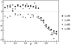
Fig. 7. The shape parameter ![]() of
skew normal distribution as a function of
of
skew normal distribution as a function of ![]() for
different system sizes
for
different system sizes
3.2. Sudden loading
In this subsection
we analyse probabilities of breakdown (![]() ) of
systems loaded by finite force
) of
systems loaded by finite force ![]() . Application of
. Application of ![]() allows us to compare results for
different system sizes. Figure 8 depicts empirical breakdown probabilities for
chosen values of weight parameter
allows us to compare results for
different system sizes. Figure 8 depicts empirical breakdown probabilities for
chosen values of weight parameter ![]() . It is seen that
fitted curves are ordered according to
. It is seen that
fitted curves are ordered according to ![]() . In
addition, the distance (in the
. In
addition, the distance (in the ![]() -direction) between
consecutive curves seems to increase as
-direction) between
consecutive curves seems to increase as ![]() is
increased. For
is
increased. For ![]() the fitted curves sharply
increase, whereas for
the fitted curves sharply
increase, whereas for ![]() and
and ![]() ,
values of
,
values of ![]() increase more slowly.
increase more slowly.
For fitting our data we employ cumulative distribution function of skew normal distribution, and thus we rewrite formula (5):
| (6) |
Figures 9-11 show
fitted values of parameters ![]() ,
, ![]() and
and ![]() for
different system sizes. It can be noticed that the behaviour of these
parameters is very similar to the behaviour of their counterparts in the case
of quasi-static loading. This proves that the two applied loading procedures
are equivalent.
for
different system sizes. It can be noticed that the behaviour of these
parameters is very similar to the behaviour of their counterparts in the case
of quasi-static loading. This proves that the two applied loading procedures
are equivalent.
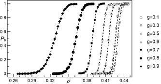
Fig. 8. Empirical breakdown probability ![]() as a function of initial load per pillar
as a function of initial load per pillar ![]() for different values of weight parameter
for different values of weight parameter ![]() . All presented data are calculated from 2000
statistically independent samples. System size
. All presented data are calculated from 2000
statistically independent samples. System size ![]() . The dashed
lines represent function (6) with parameters computed from simulations
. The dashed
lines represent function (6) with parameters computed from simulations
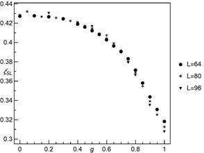
Fig. 9. The parameter ![]() of formula (6) as a
function of
of formula (6) as a
function of ![]() for different system sizes
for different system sizes
The dominance of
short range interactions is distinctly visible for ![]() (see Figures 10 and 11). The GLS regime dominates up to
(see Figures 10 and 11). The GLS regime dominates up to ![]() .
.
At the beginning
of the section, we have mentioned about distances between curves for
consecutive values of ![]() . Quartile can serve as a tool
to measure the distance in the
. Quartile can serve as a tool
to measure the distance in the ![]() -direction. Using
values of parameters
-direction. Using
values of parameters ![]() ,
, ![]() and
and ![]() we compute quartiles of the skew normal
distribution. Then we calculate differences
between quartiles for
we compute quartiles of the skew normal
distribution. Then we calculate differences
between quartiles for ![]() and for
and for ![]() . By that means we obtain distances
between consecutive curves with step of
. By that means we obtain distances
between consecutive curves with step of ![]() . The
results are plotted in Figure 12. It is seen that the distance between
consecutive curves is an increasing function up to
. The
results are plotted in Figure 12. It is seen that the distance between
consecutive curves is an increasing function up to ![]() ,
then distance start to decrease. This behaviour shows that for
,
then distance start to decrease. This behaviour shows that for ![]() short range interactions in the system
are so prevalent that further increase of
short range interactions in the system
are so prevalent that further increase of ![]() is
less
significant.
is
less
significant.
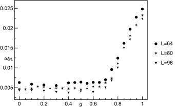
Fig. 10. The
parameter ![]() of formula (6) as a function of
of formula (6) as a function of ![]() for different system sizes
for different system sizes

Fig. 11. The
parameter ![]() of formula (6) as a function of
of formula (6) as a function of ![]() for different system sizes
for different system sizes
Finally, we
compare approximations of ![]() by cumulative
distribution functions of two distributions, namely normal and skew normal. To
study the quality of
approximation we apply the mean absolute error (MAE). The results of MAE are
reported in Figure 13. Up to
by cumulative
distribution functions of two distributions, namely normal and skew normal. To
study the quality of
approximation we apply the mean absolute error (MAE). The results of MAE are
reported in Figure 13. Up to ![]() both of the
functions generate almost equal errors (GLS regime), then mean absolute errors
for normal distribution are greater than their skew-normal counterparts (LLS
behaviour). From
both of the
functions generate almost equal errors (GLS regime), then mean absolute errors
for normal distribution are greater than their skew-normal counterparts (LLS
behaviour). From ![]() the difference is becoming
considerable and thus suggesting distinct LLS regime.
the difference is becoming
considerable and thus suggesting distinct LLS regime.
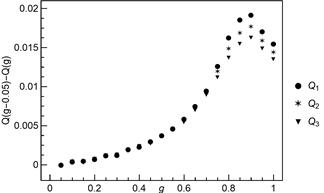
Fig. 12. The
results of subtracting quartile of SND for ![]() from
quartile of SND for
from
quartile of SND for ![]() . Parameters of SND are based
on the simulation results. The results concern systems with
. Parameters of SND are based
on the simulation results. The results concern systems with ![]() pillars
pillars
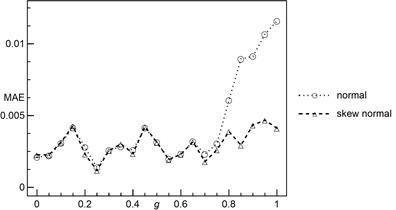
Fig. 13. Mean absolute errors of ![]() approximation using: CDF of
the SND and CDF of the normal distribution. The results concern systems with
approximation using: CDF of
the SND and CDF of the normal distribution. The results concern systems with ![]() pillars
pillars
4. Conclusions
By means of
numerical simulation, we have studied breakdown processes in the mixed-mode
load transfer model of nanopillar arrays subjected to external load. This model
is completely GLS scheme for weight parameter ![]() and pure LLS
scheme for
and pure LLS
scheme for ![]() .
.
Application of two
different loading procedures allowed us to analyse two quantities i.e. critical
load and breakdown probability. We have shown that distribution of critical
load can be nicely fitted by the skew normal distribution, and breakdown
probability is well approximated by the cumulative distribution function of
this distribution. The parameters of the these functions can serve as the
indicators of the system regime. We have tuned values of ![]() from 0 to 1 with step of 0.05. We have observed that up to
from 0 to 1 with step of 0.05. We have observed that up to ![]() long range interactions prevail (GLS
behaviour), whereas from
long range interactions prevail (GLS
behaviour), whereas from ![]() we see distinct LLS
behaviour with short range interactions. Between the two mentioned above values
of
we see distinct LLS
behaviour with short range interactions. Between the two mentioned above values
of ![]() , the crossover regime is present.
, the crossover regime is present.
In the future work we are planning to investigate critical loads and breakdown probabilities in the heterogeneous load sharing model proposed by Biswas and Chakrabarti [12]. In this model, the system is divided into two groups of elements in which part of the elements is characterised by completely local behaviour and the rest follows the global load sharing scheme which means that it is also an interpolation scheme between LLS and GLS.
References
[1] Hansen A., Hemmer P.C., Pradhan S., The Fiber Bundle Model: Modeling Failure in Materials, Wiley, 2015.
[2] Alava M.J., Nukala P.K.V.V., Zapperi S., Statistical models of fracture, Adv. in Physics 2006, 55, 349-476.
[3] Pradhan S., Hansen A., Chakrabarti B.K., Failure processes in elastic fiber bundles, Rev. Mod. Phys. 2010, 82, 499-555.
[4] Pradhan S., Chakrabarti B.K., Hansen A., Crossover behavior in a mixed-mode fiber bundle model, Phys. Rev. E 2005, 71, 036149.
[5] McCartney L.N., Smith R.L., Statistical theory of the strength of fiber bundles, J. Appl. Mech. 1983, 50(3), 601-608.
[6] Smith R.L., The asymptotic distribution of the strength of a series-parallel system with equal load-sharing, The Annals of Probability 1982, 10(1), 137-171.
[7] Porwal P.K., Beyerlein I.J., Phoenix S.L., Statistical strength of a twisted fiber bundle: an extension of Daniels equal-load-sharing parallel bundle theory, Journal of Mechanics of Materials and Structures 2006, 1(8), 1425-1447.
[8] Domański Z., Derda T., Sczygiol N., Critical Avalanches in Fiber Bundle Models of Arrays of Nanopillars, Proceedings of the International MultiConference of Engineers and Computer Scientists 2013, Vol. II, IMECS 2013, March 13-15, 2013.
[9] Derda T., Stochastic local load redistribution in the fibre bundle model of nanopillar arrays, J. Appl. Math. Comput. Mech. 2015, 14(4), 19-30.
[10] Domański Z., Derda T., Distributions of Critical Load in Arrays of Nanopillars, Proceedings of the World Congress on Engineering (WCE 2017), Vol. II, 797-801.
[11] Derda T., Avalanche statistics in transfer load models of evolving damage, Scientific Research of the Institute of Mathematics and Computer Science 2011, 10(1), 21-31.
[12] Biswas S., Chakrabarti B.K., Crossover behaviors in one and two dimensional heterogeneous load sharing fiber bundle models, Eur. Phys. J. B 2013, 86, 160.