Study of base pressure behavior in a suddenly expanded duct at supersonic Mach number regimes using statistical analysis
Jaimon D. Quadros
,S.A. Khan
,A.J. Antony
Journal of Applied Mathematics and Computational Mechanics |
 Download Full Text |
 View in HTML format |
 Export citation |
@article{Quadros_2018,
   doi = {10.17512/jamcm.2018.4.07},
   url = {https://doi.org/10.17512/jamcm.2018.4.07},
   year = 2018,
   publisher = {The Publishing Office of Czestochowa University of Technology},
   volume = {17},
   number = {4},
   pages = {59--72},
   author = {Jaimon D. Quadros and  S.A. Khan and  A.J. Antony},
   title = {Study of base pressure behavior in a suddenly expanded duct at supersonic Mach number regimes using statistical analysis},
   journal = {Journal of Applied Mathematics and Computational Mechanics}
}
TY - JOUR DO - 10.17512/jamcm.2018.4.07 UR - https://doi.org/10.17512/jamcm.2018.4.07 TI - Study of base pressure behavior in a suddenly expanded duct at supersonic Mach number regimes using statistical analysis T2 - Journal of Applied Mathematics and Computational Mechanics JA - J Appl Math Comput Mech AU - Quadros, Jaimon D. AU - Khan, S.A. AU - Antony, A.J. PY - 2018 PB - The Publishing Office of Czestochowa University of Technology SP - 59 EP - 72 IS - 4 VL - 17 SN - 2299-9965 SN - 2353-0588 ER -
Quadros, J., Khan, S., & Antony, A. (2018). Study of base pressure behavior in a suddenly expanded duct at supersonic Mach number regimes using statistical analysis. Journal of Applied Mathematics and Computational Mechanics, 17(4), 59-72. doi:10.17512/jamcm.2018.4.07
Quadros, J., Khan, S. & Antony, A., 2018. Study of base pressure behavior in a suddenly expanded duct at supersonic Mach number regimes using statistical analysis. Journal of Applied Mathematics and Computational Mechanics, 17(4), pp.59-72. Available at: https://doi.org/10.17512/jamcm.2018.4.07
[1]J. Quadros, S. Khan and A. Antony, "Study of base pressure behavior in a suddenly expanded duct at supersonic Mach number regimes using statistical analysis," Journal of Applied Mathematics and Computational Mechanics, vol. 17, no. 4, pp. 59-72, 2018.
Quadros, Jaimon D., S.A. Khan, and A.J. Antony. "Study of base pressure behavior in a suddenly expanded duct at supersonic Mach number regimes using statistical analysis." Journal of Applied Mathematics and Computational Mechanics 17.4 (2018): 59-72. CrossRef. Web.
1. Quadros J, Khan S, Antony A. Study of base pressure behavior in a suddenly expanded duct at supersonic Mach number regimes using statistical analysis. Journal of Applied Mathematics and Computational Mechanics. The Publishing Office of Czestochowa University of Technology; 2018;17(4):59-72. Available from: https://doi.org/10.17512/jamcm.2018.4.07
Quadros, Jaimon D., S.A. Khan, and A.J. Antony. "Study of base pressure behavior in a suddenly expanded duct at supersonic Mach number regimes using statistical analysis." Journal of Applied Mathematics and Computational Mechanics 17, no. 4 (2018): 59-72. doi:10.17512/jamcm.2018.4.07
STUDY OF BASE PRESSURE BEHAVIOR IN A SUDDENLY EXPANDED DUCT AT SUPERSONIC MACH NUMBER REGIMES USING STATISTICAL ANALYSIS
Jaimon D. Quadros 1, S.A. Khan 2, A.J. Antony 3
1
Department of Mechanical Engineering, Birla Institute of Technology, Offshore
campus
Ras-Al-Khaimah, UAE
2 Department of Mechanical Engineering, International Islamic
University Malaysia
Kuala Lampur, Malaysia
3 Department of Mechanical Engineering, Bearys Institute of
Technology
Mangalore, India
jaimonq@gmail.com, sakhan06@gmail.com, aajsit@gmail.com
Received: 13 March 2018; Accepted: 18 December 2018
Abstract. The present experimental evaluation deals with the behavior of base pressure (BP) in a suddenly expanded duct at supersonic Mach number regimes. The experiments have been conducted for two cases viz. Without and with the use of microjets or active control. The plan of experiments was planned as per Taguchi design of experiments for acquiring data in a controlled manner. An L27 orthogonal array and analysis of variance (ANOVA) has been employed to investigate the contribution (in terms of percentage) of distinct process parameters like Mach number (M), Nozzle Pressure Ratio (N), Area Ratio (A) and their interactions affecting base pressure. The correlation between these parameters affecting base pressure has been obtained using multiple linear regression analysis. It has been concluded that the Mach number and area ratio were the factors that had high statistical significance on the behavior of base pressure for both cases. The performances of the developed linear regression models have been validated for accuracy prediction by use of 15 test cases. The performance of both the base pressure models was found to be better with percentage prediction in deviation lying in the range of –12.92% to +15.88% for base pressure without control and –10.27% to +19.23% for base pressure with control.
MSC 2010: 34B60, 82-08
Keywords: Mach number, Taguchi, nozzle pressure ratio, area ratio
1. Introduction
In the wake of developments in space technology and missiles, the study of base flows at a high Reynolds number remains to be a prime area of research. It is well known in previous literature that base pressure can be as high as 50 percent of the total drag during off jet conditions. However, during jet on conditions, the pressure at the base tends to be high due to negligible suction [1, 2]. Thus the base pressure and consequently base drag can be controlled in the case of blunt projectiles thereby leading to a considerable increase in the range of missiles and projectiles. As far as friction drag and wave drag are concerned, considerable work has already been conducted and reported leaving little scope for further investigation. Thus optimization and control of base pressure is the only area of exploration currently available. The major objectives of the present study are to optimize and control the base pressure required for smooth flow development without oscillations and to also minimize the total pressure gradient. Therefore, the experiments in the present study are conducted in an enlarged duct in order to ensure no negative effect of control on the duct flow field.
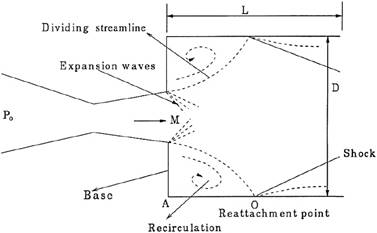
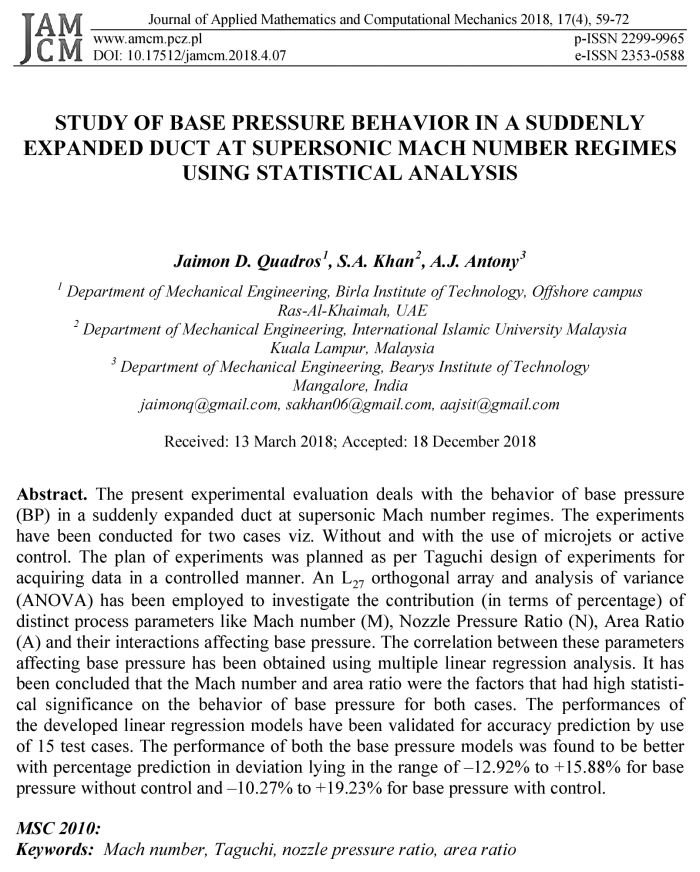
Fig. 1. Suddenly expanded flow field
A flow field in a suddenly expanded duct is a variegated phenomenon characterized by flow separation, flow recirculation and flow reattachment. The flow field is divided into two regions by the shear layer i.e. the recirculation region and the main flow region. The point where the divided streamlines strike the wall is referred to as the reattachment point. The features of a suddenly expanded flow field [3] are shown in Figure 1. The desired testing of parameters in done either by experience or by use of a handbook. However, it does not provide the optimal parameter for a particular situation. There are numerous mathematical models based on statistical regression techniques that are constructed for proper selection of testing conditions. Taguchi’s design of experiments is an effective and systematic approach to optimize the performance, quality and cost of a design [4]. Taguchi’s design can be streamlined by expending the application of the traditional experimental designs to the use of orthogonal array. Below are a few works of scientists having taken up the problems relating to base pressure control and optimization. Chapman et al. [5] initially conducted experiments on base pressure in order to study its effects on a boundary layer. He concluded that base pressure is directly correlated to boundary layer thickness and location of the transition point. Tanner [6] studied a base cavity at different angles of incidence. He concluded that a base cavity could increase the base pressure and thus decrease the base drag in an axi-symmetric flow. He varied the angle of incidence from 0 to 250. The maximum drag reduction was found at α = 20. The reduction of base drag at Mach 2 was studied by Viswanath [7]. He employed passive devices for this purpose. The devices hired possessed base cavities and ventilated cavities. The results showed that ventilated cavities displayed significant reduction in base drag of about 50 percent. Rathakrishnan [8] experimentally investigated the influence of cavities on a suddenly expanded subsonic flow field. They studied base pressure variation through a convergent axi-symmetric nozzle expanding suddenly into an annular shroud consisting of annular cavities. Khan et al. [9-13] conducted experimental investigations in order to study the influence of microjets for controlling base pressure in a suddenly expanded axisymmetric duct. It was found that the microjets serve as controllers for increasing base pressure for a combination of parameters. The maximum increase in base pressure was 152 percent. Furthermore, it was also concluded that Mach number and nozzle pressure ratio play a definitive role in deciding the base pressure without and with the use of microjets. Based on the literature cited above, very little importance has been given towards optimization of flow control and its effectiveness. Therefore, it was thought worthwhile to conduct the above study as it will be of immense help for various rocket and space programs wherein the behavior of the base pressure is to be understood fully, since base pressure control will result in either an increase or decrease in base pressure.
Nozzles come up in a vast range of applications. Obvious ones are the thrust nozzles of rocket and jet engines. Converging-diverging ducts also come up in aircraft engine inlets, wind tunnels and in all sorts of piping systems designed to control gas flow. The flows associated with volcanic and geyser eruptions are influenced by converging-diverging nozzle geometries that arise naturally in geological formations. From area-averaged equations of motion [14], by neglecting the shear stresses and heat fluxes, the governing equations together with the perfect gas law can be expressed in fractional differential form as
| (1) |
| (2) |
| (3) |
| (4) |
Equation for a Mach number fractional differential form can be expressed as
| (5) |
By using the equations for mass, momentum and energy to replace the terms in the equation of state, we get
| (6) |
Equation (6) shows the effect of stream wise
area change on the speed of the flow. Using
Eq. (6) to replace ![]() in each of the relations in Eqs. (1),
(2) and (3), we get:
in each of the relations in Eqs. (1),
(2) and (3), we get:
| (7) |
| (8) |
| (9) |
Equations (7), (8) and (9) describe the effects of area change on the thermodynamic state of the flow. Using Eq. (9) in Eq. (6) by rearranging and integrating from the initial Mach number to 1, we get,
 | (10) |
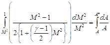
Evaluating equation at the limits, we get
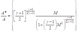 | (11) |
In the above equation, we referenced the integration process to M = 1. The area A* is a reference area at some point in the channel where M = 1 although such a point need not actually be present in a given problem. The area-Mach-number function is given by equation (11).
2. Plan of experiments
The experiments were conducted as per the Taguchi Design of Experiments. The orthogonal array is selected based on the condition that the degree of freedom of the array should be greater than the sum of the flow parameters. Therefore a standard L27 orthogonal array was implemented [15]. This array consists of 27 rows and 13 columns. The first column was assigned to Mach number (M), the second column was assigned to Nozzle Pressure Ratio (N), the fifth column was assigned to Area ratio (A) and the remaining columns were assigned to their interactions. The response to be studied was the base pressure without and with the use of microjets. The process parameters and their levels are shown in Table 1.
Table 1. Process parameters and their levels
|
Levels |
Mach number (M) |
Nozzle pressure ratio (N) |
Area ratio (A) |
|
1 |
2.0 |
5 |
3.24 |
|
2 |
2.5 |
7 |
4.84 |
|
3 |
3.0 |
9 |
6.25 |
3. Experimental setup
The experimental set up is shown in Figure 2. The set up consists of a nozzle with eight holes at its exit periphery out of which, four (marked c) were used for blowing and the remaining four (marked m) were used for measuring base pressure. The base pressure was regulated through the control holes (c), by use of a settling chamber by employing a tube which connects the settling chamber with the control holes. The experiments were conducted for a suddenly expanded duct for a length to diameter (l/d) ratio of 4.
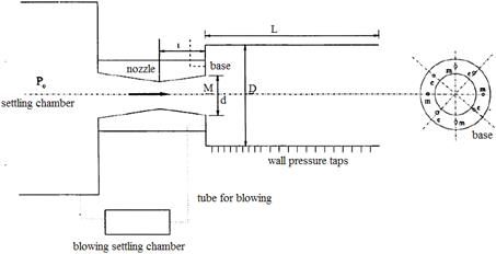
Fig. 2. Experimental set up
A PSI model 9010 pressure transducer was used for measuring base pressure and pressure in the settling chamber. It measures pressure ranging from 0 to 300 psi. The readings are averaged at the rate of 250 samples per second and displayed. The computer and the transducer were interfaced by user-friendly software. The software acquires data from all the base pressure measuring channels and simultaneously displays it on the computer screen. The system is operated in temperatures ranging from –20 to +60° and 95% humidity. The transducer had a measurement resolution of ±0.003 and the readings were accurate up to ±1 per cent.
4. Results and discussions
The experiments were conducted with an aim of relating the influence of Mach number (M), nozzle pressure ratio (N) and Area ratio (A) on base pressure behavior of suddenly expanded flows with and without the use of microjets. On conducting the experiments as per the orthogonal array, the base pressure results for various combinations of parameters have been obtained and shown in Table 2. The results indicate that the use of control or microjets do not influence the flow field adversely as the base pressure values for both the cases are pretty similar.
Table 2. Experimental results for Taguchi L27 (313) array for base pressure without and with the use of active control
|
S.I. No. |
M |
N |
A |
BP (WoC) |
BP (WC) |
|
1 |
2.0 |
3 |
3.24 |
0.606 |
0.603 |
|
2 |
2.0 |
3 |
4.84 |
0.699 |
0.699 |
|
3 |
2.0 |
3 |
6.25 |
0.754 |
0.760 |
|
4 |
2.0 |
7 |
3.24 |
0.121 |
0.140 |
|
5 |
2.0 |
7 |
4.84 |
0.18 |
0.174 |
|
6 |
2.0 |
7 |
6.25 |
0.536 |
0.381 |
|
7 |
2.0 |
11 |
3.24 |
0.216 |
0.240 |
|
8 |
2.0 |
11 |
4.84 |
0.143 |
0.170 |
|
9 |
2.0 |
11 |
6.25 |
0.091 |
0.120 |
|
10 |
2.5 |
3 |
3.24 |
0.714 |
0.722 |
|
11 |
2.5 |
3 |
4.84 |
0.793 |
0.793 |
|
12 |
2.5 |
3 |
6.25 |
0.838 |
0.840 |
|
13 |
2.5 |
7 |
3.24 |
0.471 |
0.425 |
|
14 |
2.5 |
7 |
4.84 |
0.575 |
0.562 |
|
15 |
2.5 |
7 |
6.25 |
0.614 |
0.620 |
|
16 |
2.5 |
11 |
3.24 |
0.061 |
0.081 |
|
17 |
2.5 |
11 |
4.84 |
0.076 |
0.068 |
|
18 |
2.5 |
11 |
6.25 |
0.567 |
0.554 |
|
19 |
3.0 |
3 |
3.24 |
0.845 |
0.850 |
|
20 |
3.0 |
3 |
4.84 |
0.889 |
0.890 |
|
21 |
3.0 |
3 |
6.25 |
0.908 |
0.912 |
|
22 |
3.0 |
7 |
3.24 |
0.643 |
0.634 |
|
23 |
3.0 |
7 |
4.84 |
0.709 |
0.720 |
|
24 |
3.0 |
7 |
6.25 |
0.766 |
0.770 |
|
25 |
3.0 |
11 |
3.24 |
0.542 |
0.550 |
|
26 |
3.0 |
11 |
4.84 |
0.614 |
0.597 |
|
27 |
3.0 |
11 |
6.25 |
0.662 |
0.652 |
4.1. ANOVA and effect of factors
Analysis of variation (ANOVA) is carried out to statistically test significance of the combined effect of all linear, square and interaction factors and the adequacy of developed models. The ANOVA allows one to analyze the influence of each variable on the total variance of the results. This is done by comparing the means between the variables and determines whether any of these means are statistically significantly different from each other [16]. Statistically, there is a tool called an F test, named after Fisher, to see which design parameters have a significant effect on the quality characteristic. In the analysis, the F-ratio is a ratio of the mean square error to the residual error and is traditionally used to determine the significance of a factor. The P (%) reports the significance level (suitable and unsuitable). Table 3 shows the results of ANOVA for base pressure without control or without the use of microjets. The level of significance i.e. level of confidence used for the performance of analysis was 95%. The last column in the table represents the significance/ influence level or percentage contribution % (P) of each parameter affecting the response variable i.e. base pressure. If the ”Test F” value is greater than the F (1%) column value, then the assigned variable is statistically significant.
Table 3. Analysis of variance (ANOVA) for base pressure results without the use of active control
|
Source |
DF |
SS |
Variances |
Test F |
F |
Pa(%) |
|
M |
2 |
24.22 |
12.11 |
16.39 |
9a |
30.07 |
|
N |
2 |
38.65 |
19.32 |
26.46 |
19a |
47.98 |
|
A |
2 |
5.56 |
2.78 |
3.80 |
9a |
6.91 |
|
M*N |
4 |
4.36 |
1.09 |
1.48 |
4a |
5.42 |
|
M*A |
4 |
1.03 |
0.25 |
0.35 |
4a |
1.29 |
|
N*A |
4 |
0.78 |
0.20 |
0.27 |
4a |
0.97 |
|
Error |
8 |
5.90 |
0.73 |
– |
– |
7.33 |
|
Total |
26 |
80.56 |
– |
– |
– |
100 |
Table 4. Analysis of variance (ANOVA) for base pressure results with the use of active control
|
Source |
DF |
SS |
MS |
Test F |
F |
P(%) |
|
M |
2 |
26.17 |
13.08 |
25.75 |
9a |
31.75 |
|
N |
2 |
40.36 |
20.18 |
39.71 |
19a |
48.96 |
|
A |
2 |
4.67 |
2.33 |
4.60 |
9a |
5.67 |
|
M*N |
4 |
5.04 |
1.26 |
2.48 |
4a |
6.12 |
|
M*A |
4 |
1.41 |
0.35 |
0.70 |
4a |
1.72 |
|
N*A |
4 |
0.49 |
0.12 |
0.34 |
4a |
0.60 |
|
Error |
8 |
4.03 |
0.50 |
– |
– |
4.90 |
|
Total |
26 |
82.44 |
– |
– |
– |
100 |
It can be clearly observed from Table 3 that nozzle pressure ratio (P = 47.98%), Mach number (P = 30.07%), area ratio (P = 6.91%) and interactions between Mach number/nozzle pressure ratio (P = 5.42%) has great influence on base pressure without active control. Mach number/area ratio (P = 1.29%) and nozzle pressure ratio/area ratio (P = 0.97%) does not have a significant effect (both physical and statistical) on the base pressure without active control and are consequently neglected. The error associated in the ANOVA table is about 7.33%. The ANOVA for base pressure with active control has been shown in Table 4. It is observed that nozzle pressure ratio (P = 48.96%) is the major factor influencing base pressure with control followed by Mach number (P = 31.75%) and area ratio (P = 5.67%). On the other hand, interactions between Mach number/nozzle pressure ratio (P = 6.12%) Mach number/ area ratio (P = 1.72%) and nozzle pressure ratio/area ratio (P = 0.60%) exert no influence on the base pressure without the use of microjets. The error associated in the ANOVA table is about 4.60%.
Here, in both cases, it is observed that nozzle pressure ratio had maximum impact on base pressure among the tested variables. As the nozzle pressure ratio increases, the level of overexpansion comes down; hence the oblique shock at the nozzle exit becomes weaker. Therefore the turning away tendency of the incoming flow decreases leaving the vortex almost intact. In this situation, when micro jets are introduced, they may propagate without any deflecting tendency, thereby entraining some mass from the standing vortex and convecting it away from the base causing the base pressure to assume higher values than for those without control case [16]. The Mach number also influences base pressure significantly. This is because Mach numbers of the jets at Mach 2.5 and 3.0 experience a high over expansion where a stronger effect at the nozzle exit is experienced causing a significant change in base pressure [17]. It can be clearly noted that the term area ratio also plays an important role in influencing base pressure, especially in secondary flows near duct corners. For a particular area ratio, for a given Mach number and nozzle pressure ratio, there is a transverse pressure gradient, which provides the centripetal force for the secondary fluid elements to change direction. This results in the fluid near the nozzle exit moving outwards and the fluid near the corner walls moving inwards [18]. As the area ratio increases, the secondary vortices that are attached to the horizontal walls become stronger and reach farther in the spanwise and vertical directions [19, 20]. Consequently, their counter-rotating neighbors in the adjacent vertical straight walls become weaker and increasingly attached to the wall leading to an increase in base pressure.
The main effect plots for base pressure without and with control are shown in Figures 3 and 4 respectively. It can be clearly observed that the main effect plots for base pressures without and with control are very similar in nature. This can be attributed to the fact that the use of microjets does not affect the base pressure significantly as the values remain similar and are shown Table 2, referred to earlier. It can be clearly observed that an increase in the Mach number (M) experiences a significant increase in the base pressure followed by area ratio (A) which shows a considerably smaller increase in base pressure. However, with the increase on nozzle pressure ratio (N), the base pressure saw a steep decrease. Thus from Figures 3 and 4, it can be inferred that the nozzle pressure ratio has the highest significance on optimal setting conditions, followed by Mach number. The influence of area ratio shows a lesser effect on base pressure variation as it contributes to a comparatively smaller extent when compared to the rest of the parameters.
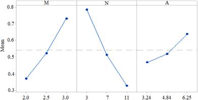
Fig. 3. Main effect plots for base pressure results without the use of active control
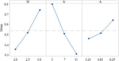
Fig. 4. Main effect plots for base pressure results with the use of active control
4.2. Regression analysis
A linear regression technique has been implemented to study the base pressure in a suddenly expanded duct. The general expression for regression is given by
| Y = a0 + a1X1 + a2X2 + a3X3 + a4X1X2 + a5X3X1 + a6X2X3 + a7X1X2X3 | (12) |
In the above equation (12), Y represents the response base pressure. The variables X1, X2 and X3 represent the Mach number, nozzle pressure ratio and area ratio respectively. The terms a1, a2 and a3 represent the coefficients of the independent variable i.e. X1, X2 and X3 respectively. The a4, a5, a6, and a7 are the interaction coefficients between X1X2, X1X3, X2X3 and X1X2X3 respectively, within the selected levels of each of the variables. The above expression in its basic form is
| Yi = a0 + a1X1i + a2X2i + ... + aiXpi | (13) |
In equation (13), the intercept, a0 of the line, gives the expected value of Y when all x’s = 0. The slopes, aj, j = 1...p where p is the number of explanatory variables, (for our case j = 1….7) give the increase (or decrease) in Y for a unit increase in each xji, given the other explanatory variables in the model. After calculating each of the coefficients of equation (12), the final linear regression equation for the base pressure is obtained. The regression equation for base pressure without control and with control is
| Y1 = –0.89 + 0.655 M + 0.016 N + 0.315 A – 0.0329 M×N – 0.110 M×A – 0.0322 N×A + 0.0137 M×N×A | (14) |
| Y2 = –0.74 + 0.594 M + 0.024 N + 0.263 A – 0.0346 M×N – 0.089 M×A – 0.0315 N×A + 0.0132 M×N×A | (15) |
In the equations (14) and (15), Y1 and Y2 represent base pressure with and without control respectively. The coefficients of determination (R2) for base pressure without and with control are 87.19 and 88.58% respectively. The behavior of base pressure with control is found to be more accurate than without control. The value of a0 for base pressure without and with control is –0.89 and –0.74 respectively. The value of a0 is the intercept of the plane and is a mean response value for all experiments conducted. This value not only depends on parameters like M, N and A; but also takes irregular parameters into account like experimental irregularities, flow losses, environmental conditions, surface roughness of the ducts etc. [21, 22].
4.3. Confirmation tests
The confirmation tests have been conducted to validate the statistical analysis by conducting experiments on base pressure for the same parameters, but are however different from those used for analysis as shown earlier in Table 2. Table 5 shows the experimental conditions for the confirmation tests performed. The estimations of percentage deviation in prediction are found to lie in the range of –12.92% to +15.88% for the case of base pressure without control (Fig. 5a) and in the range of –10.27% to +19.23% for base pressure with control (Fig. 5b). The base pressure was successfully predicted with a root mean square error RMSE = 0.0037 for without control and RMSE = 0.0039 for with control respectively.
Table 5. Confirmation tests
|
Test No. |
M |
N |
A |
BP (WoC) |
BP (WC) |
|
1. |
2.5 |
5 |
3.25 |
0.476 |
0.460 |
|
2. |
3 |
7 |
3.25 |
0.595 |
0.573 |
|
3. |
3 |
7 |
4.75 |
0.699 |
0.671 |
|
4. |
2.5 |
7 |
3.25 |
0.347 |
0.330 |
|
5. |
2 |
7 |
6.25 |
0.376 |
0.368 |
|
6. |
2.5 |
9 |
6.25 |
0.374 |
0.369 |
|
7. |
3 |
9 |
6.25 |
0.651 |
0.641 |
|
8. |
2 |
7 |
6.25 |
0.327 |
0.360 |
|
9. |
2.5 |
5 |
3.25 |
0.388 |
0.397 |
|
10. |
2.5 |
5 |
3.25 |
0.557 |
0.539 |
|
11. |
3 |
7 |
6.25 |
0.692 |
0.689 |
|
12. |
3 |
9 |
4.75 |
0.619 |
0.700 |
|
13. |
3 |
5 |
6.25 |
0.809 |
0.810 |
|
14. |
2.5 |
7 |
4.75 |
0.489 |
0.471 |
|
15. |
2 |
9 |
6.25 |
0.191 |
0.200 |
a)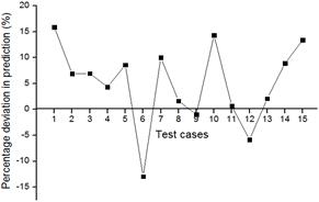 b)
b)
Fig. 5. Standard deviation in prediction of 15 test cases for: a) base pressure without active control, b) base pressure with active control
Additionally, the line of best fit is used to make the comparison. Here, the experimental values obtained are compared with those of corresponding model predicted values. It has also been observed that the best fit line obtained for the model of base pressure (WoC) as shown in Figure 6a shows noticeable deviation of data points from the ideal, y = x line. However the best fit line for the model of base pressure (WC) shown in Figure 6b shows considerably lesser deviation of data points from the ideal y-x line thereby indicating better predictability of the model when compared to the model of base pressure (WoC).
a)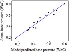 b)
b)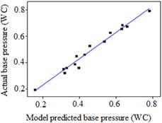
Fig. 6. Comparison of model predicted base pressure with actual base pressure for: a) base pressure without active control, b) base pressure with active control
5. Conclusions
Base pressure behavior has been studied using statistical analysis without and with the use of control or microjets. Mach number, nozzle pressure ratio and area ratio are the parameters involved in the study. The following conclusions have been drawn:
· Mach number and nozzle pressure ratio were found to have the highest physical and statistical significance on base pressure without and with control respectively. Area ratio was found to have the least significance.
· The confirmation tests showed the percentage deviation in prediction was found to lie in the range of –12.92% to +15.88% for the case of base pressure without control and in the range of –10.27% to +19.23% for base pressure with control.
· The present work presents a methodology to model and analyze the base pressure process utilizing statistical tools. Further, it will help in reducing base drag, when one needs to consider expanding base pressure to the more extreme and similarly for improvement of mixing when one needs to go for diminishing base pressure to the lowest possible value. The regression models can be used to predict the response values without conducting experiments for the set of process parameters.
NOMENCLATURE
A Area ratio R Ideal gas constant 8.314·103 (kg m2 mol−1 K−1 s−2)
A* Throat area of the nozzle T Temperature of Ideal gas
F Fisher statistic U Local flow velocity with respect to the boundaries
M Mach number γ Ratio of specific heat at constant pressure to constant N Nozzle pressure ratio volume (1.4 for air)
P Probability BP Base pressure
Pa Ambient pressure MS Mean of squares
SS Sum of squares
References
[1] Singh, N.K., & Rathakrishnan E. (2002). Sonic jet control with tabs. Journal of Turbo and Jet Engines, 19(1-2), 107-118.
[2] Anderson, J.S., & Williams, T.J. (1968). Base pressure and noise produced by the abrupt expansion of air in a cylindrical duct. Journal of Mechanical Engineering Science, 10(3), 262-268.
[3] Rathakrishnan, E., & Sreekanth, A.K. (1984). Flow in pipes with sudden enlargement. Proceedings of the 14th International Symposium on Space Technology and Science. Tokyo, Japan.
[4] Basavarajappa, S., Yadav, S.M., Kumar, S., Arun, K.V., & Narendranath, S. (2011). Abrasive wear behavior of granite-filled glass-epoxy composites by SiC particles using statistical analysis. Polymer-Plastics Technology and Engineering, 50(5), 516-524.
[5] Chapman, D.R. (1950). An analysis of base pressure at supersonic velocities and comparison with experiments, NACA TN 2137.
[6] Tanner, M. (1988). Base cavities at angles of incidence. AIAA Journal, 26(3), 376-377.
[7] Viswanath, P.R., & Patil, S.R. (1990). Effectiveness of passive devices for axi-symmetric base drags reduction at Mach 2. Journal of Spacecraft, 27(2), 234-237.
[8] Rathakrishnan, E., Ramanaraju, O.V., & Padmanabhan, K. (1989). Influence of cavities on suddenly expanded flow field. Mechanics Research Communications, 16(3), 139-146.
[9] Khan, S.A., & Rathakrishnan, E. (2006). Control of suddenly expanded flow, aircraft engineering and aerospace technology. An International Journal, 78(4), 293-309.
[10] Khan, S.A., & Rathakrishnan, E. (2004). Control of suddenly expanded flow from correctly expanded nozzles. International Journal of Turbo and Jet Engines, 21(4), 255-278.
[11] Khan, S.A., & Rathakrishnan, E. (2004). Active control of suddenly expanded flow from under expanded nozzles. International Journal of Turbo and Jet Engines, 21(4), 233-253.
[12] Khan, S.A., & Rathakrishnan, E. (2003). Control of suddenly expanded flows with micro jets. International Journal of Turbo and Jet Engines, 20(1), 63-81.
[13] Khan, S.A., & Rathakrishnan, E. (2002). Active control of suddenly expanded flows from over expanded nozzles. International Journal of Turbo and Jet Engine, 19(3), 119-126.
[14] Cantwell, B.J. (1996). Fundamentals of Compressible Flow. AA210, Department of Aeronautics and Astronautics, Stanford University, California, USA.
[15] Basavarajappa, S., Joshi, A.G., Arun, K.V., Kumar, A.P., & Kumar, M.P. (2009). Three-body abrasive wear behaviour of polymer matrix composites filled with SiC particles. Polymer-Plastics Technology and Engineering, 49(1), 8-12.
[16] Quadros, J.D., Khan, S.A., & Antony, A.J. (2018). Study of effect of flow parameters on base pressure in a suddenly expanded duct at supersonic mach number regimes using CFD and design of experiments. Journal of Applied Fluid Mechanics, 11(2), 483-496.
[17] Quadros, J.D., Khan, S.A., & Antony, A.J. (2018). Modelling of suddenly expanded flow process in supersonic mach regime using design of experiments and response surface methodology. Journal of Computational Applied Mechanics, 49(1), 149-160.
[18] Moinuddin, K.A.M., Joubert, P.N., & Chong, M.S. (2004). Experimental investigation of turbulence-driven secondary motion over a streamwise external corner. Journal of Fluid Mechanics, 511, 1-23.
[19] Perkins, H.J. (1970). The formation of streamwise vorticity in turbulent flow. Journal of Fluid Mechanics, 44, 721-740.
[20] Vinuesa, R., Prus, C., Schlatter, P., & Nagib, H.M. (2016). Convergence of numerical simulations of turbulent wall-bounded flows and mean cross-flow structure of rectangular ducts. Meccanica, 51, 3025-3042.
[21] Quadros, J.D., Khan, S.A., Antony, A.J., & Vas, J.S. (2016). Experimental and numerical studies on flow from axisymmetric nozzle flow with sudden expansion for Mach 3.0 using CFD. International Journal of Energy, Environment, and Economics, 24(1), 87-97.
[22] Quadros, J.D., Khan, S.A., & Antony, A.J. (2017). Investigation of effect of process parameters on suddenly expanded flows through an axi-symmetric nozzle for different Mach Numbers using design of experiments. IOP Conference Series: Materials Science and Engineering, 184(1), 1-8.